本文为原创文章,未经本人允许,禁止转载。转载请注明出处。
1.TensorBoard简介
TensorBoard是TensorFlow中的可视化工具包。
TensorBoard 提供机器学习实验所需的可视化功能和工具:
- 跟踪和可视化损失及准确率等指标
- 可视化模型图(操作和层)
- 查看权重、偏差或其他张量随时间变化的直方图
- 将嵌入投射到较低的维度空间
- 显示图片、文字和音频数据
- 剖析 TensorFlow 程序
- 以及更多功能
2.TensorBoard的使用
TensorBoard有很多栏目,例如:
接下来我们介绍常用的几个。
2.1.GRAPHS
我们以【Tensorflow基础】第四课:手写数字识别中的手写数字识别代码为例,代码地址:简易手写数字识别模型。
对代码做出以下修改:
建立命名空间:
1
2
3
4
5
#命名空间
with tf.name_scope("input"):
    #定义网络的输入和输出
    x=tf.placeholder(tf.float32,[None,784],name='x-input')#28*28*1=784
    y=tf.placeholder(tf.float32,[None,10],name='y-input')#0,1,2,3,4,5,6,7,8,9
添加保存网络图的代码:
1
writer=tf.summary.FileWriter("logs/",sess.graph)
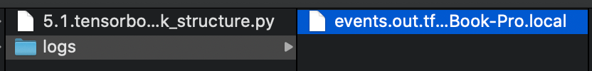
运行代码,在logs文件夹下生成了保存模型信息的文件:
打开终端,输入:tensorboard --logdir=<log_path>
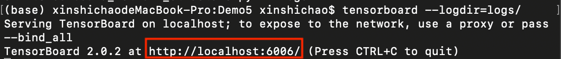
将红框中的网址粘贴到谷歌浏览器中:
关于图中一些基本符号的解释可在上图左下角处找到。
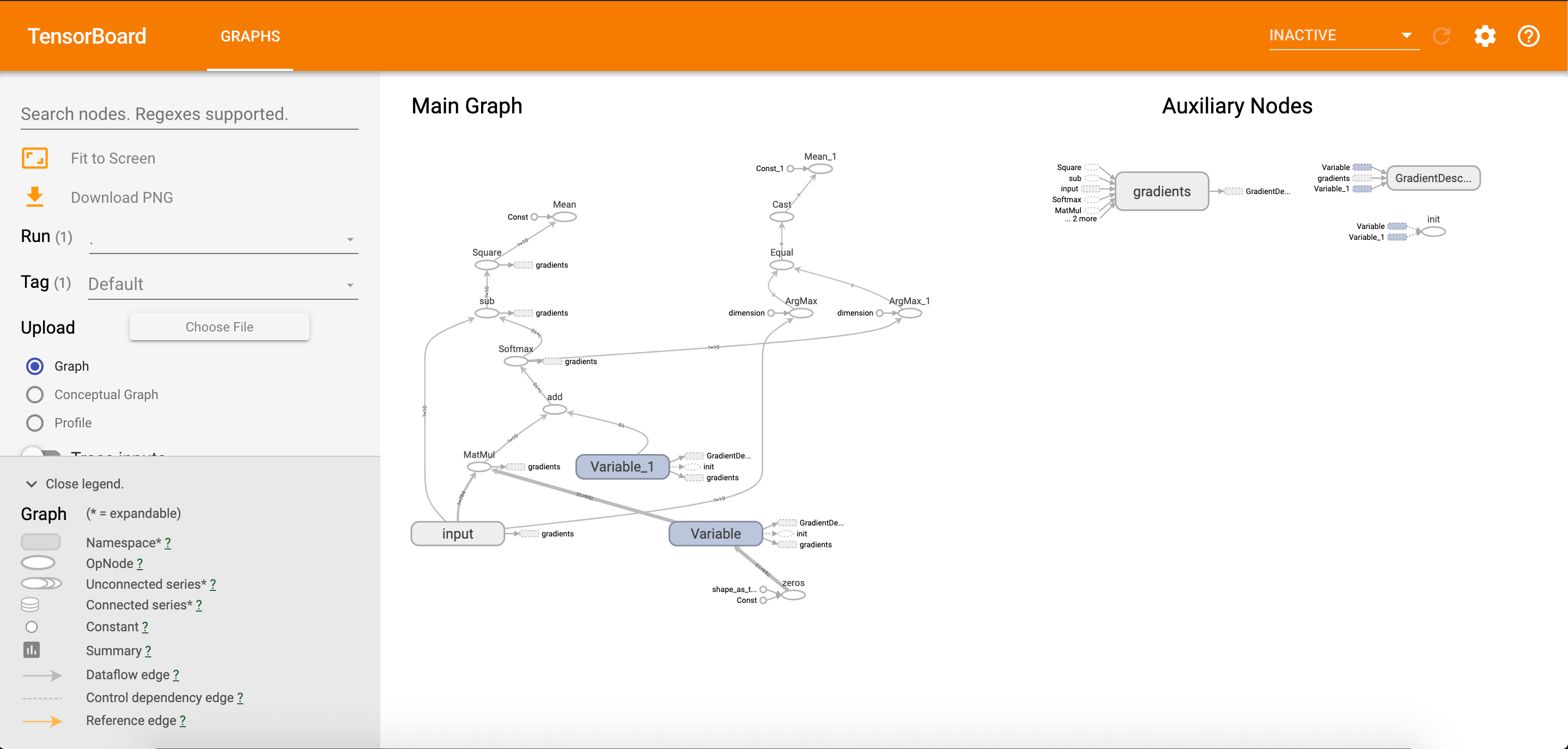
双击input(即我们之前定义的name_scope)进行查看:
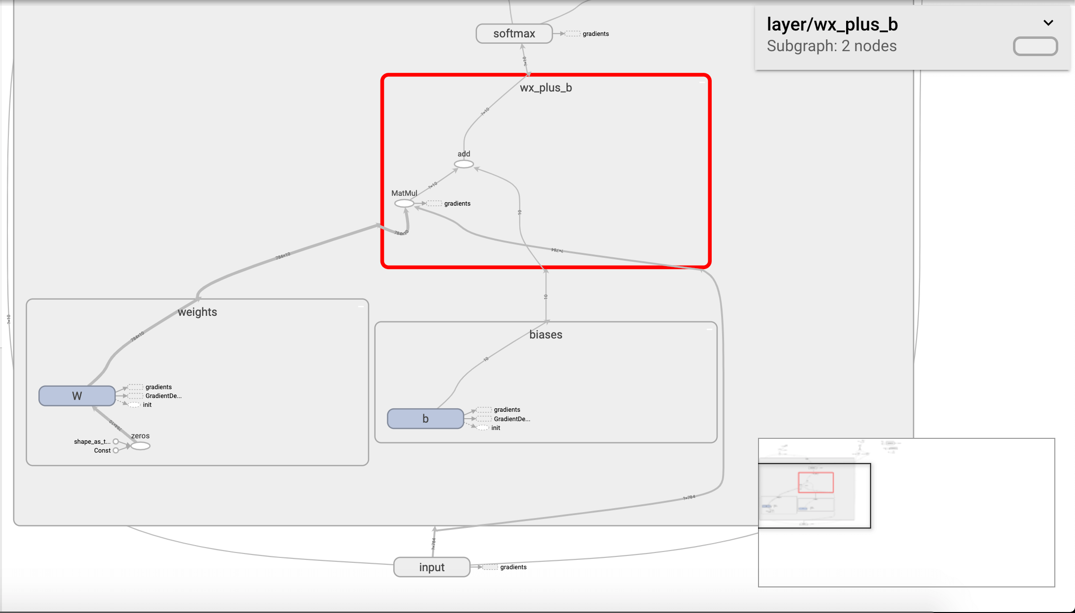
可以看到我们定义的x-input和y-input。我们也可以查看某一节点的输入和输出:
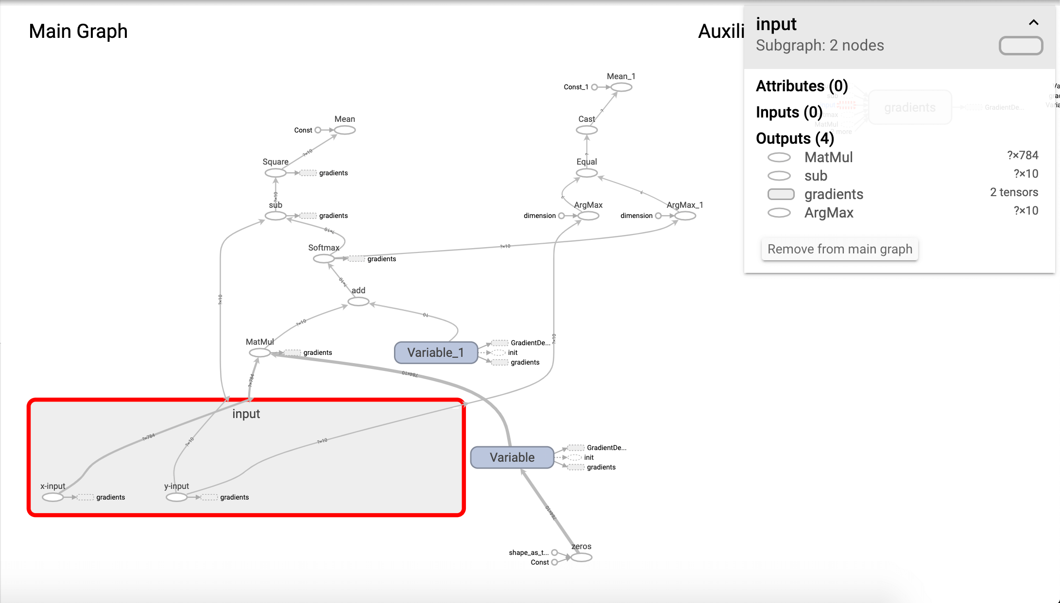
可以看到,和我们代码中定义的MatMul计算都是可以对应上的。
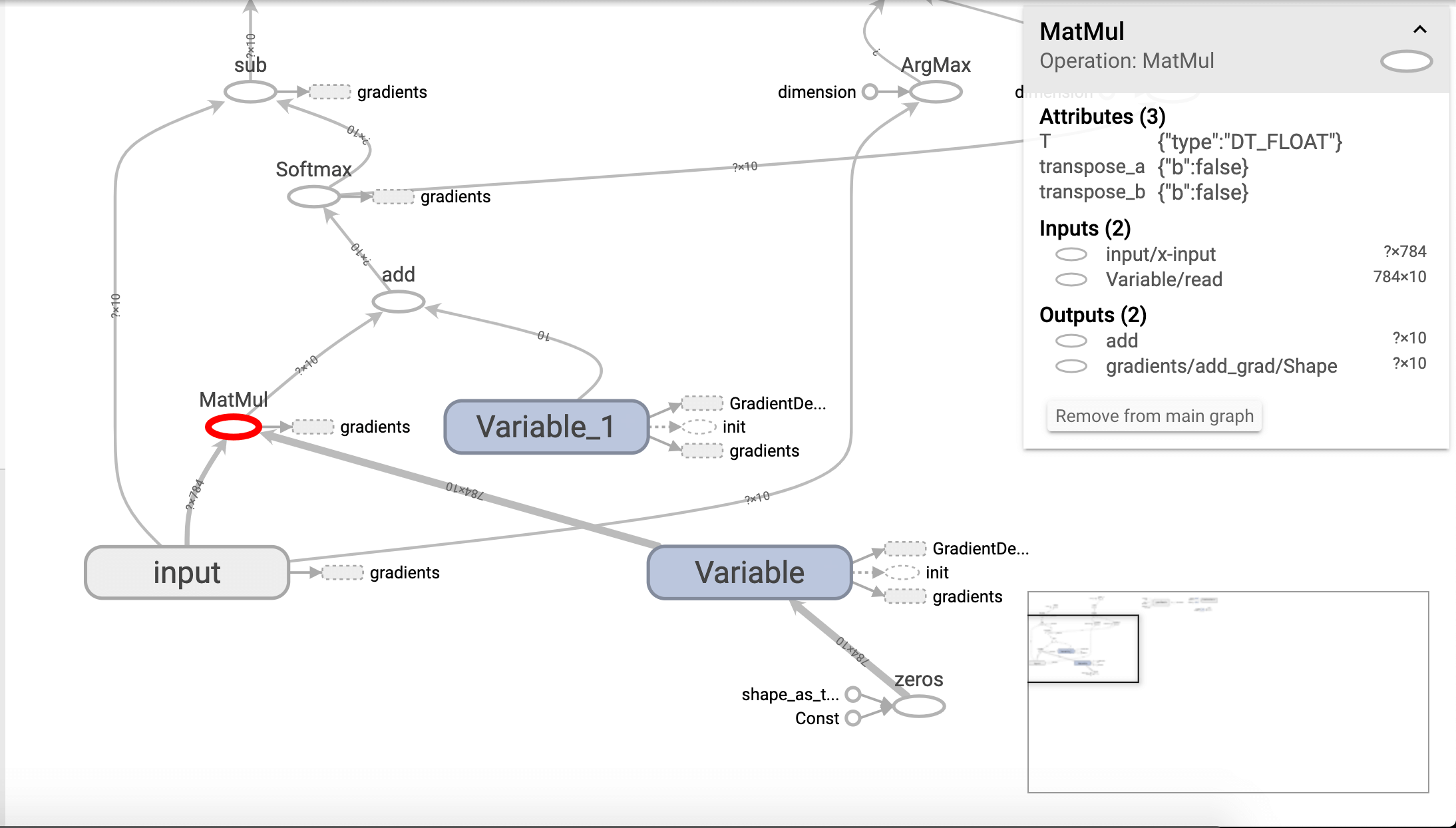
此外, 我们在图的右侧可以看到一些“孤立”的节点,这些节点实际是在主图中的,只是被抽离出来显示详细信息了而已。单击该节点即可看到其在主图中的位置:
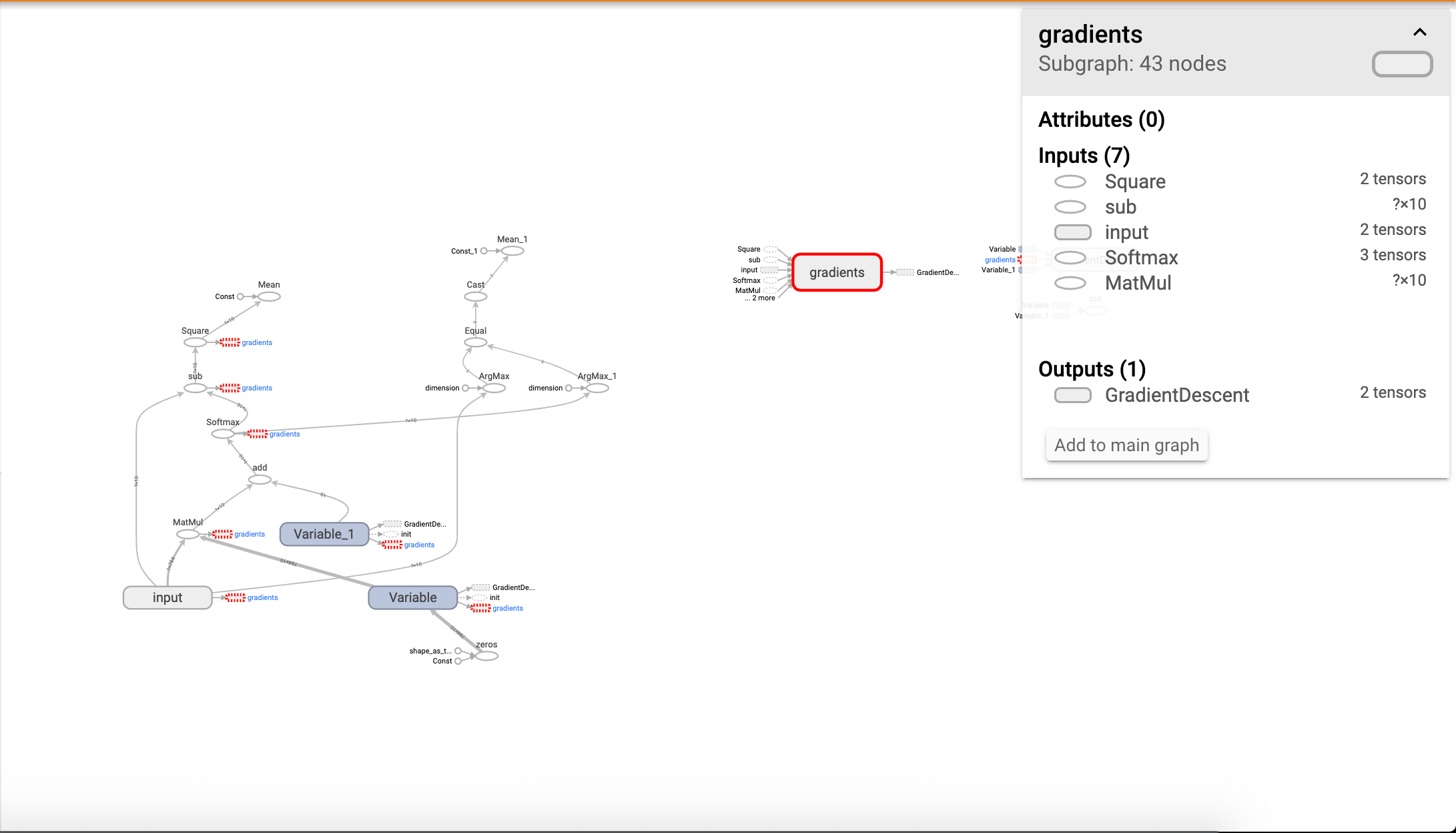
当然我们也可以选择让该节点不孤立显示,回到主图中:
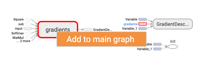
选择Add to main graph即可:
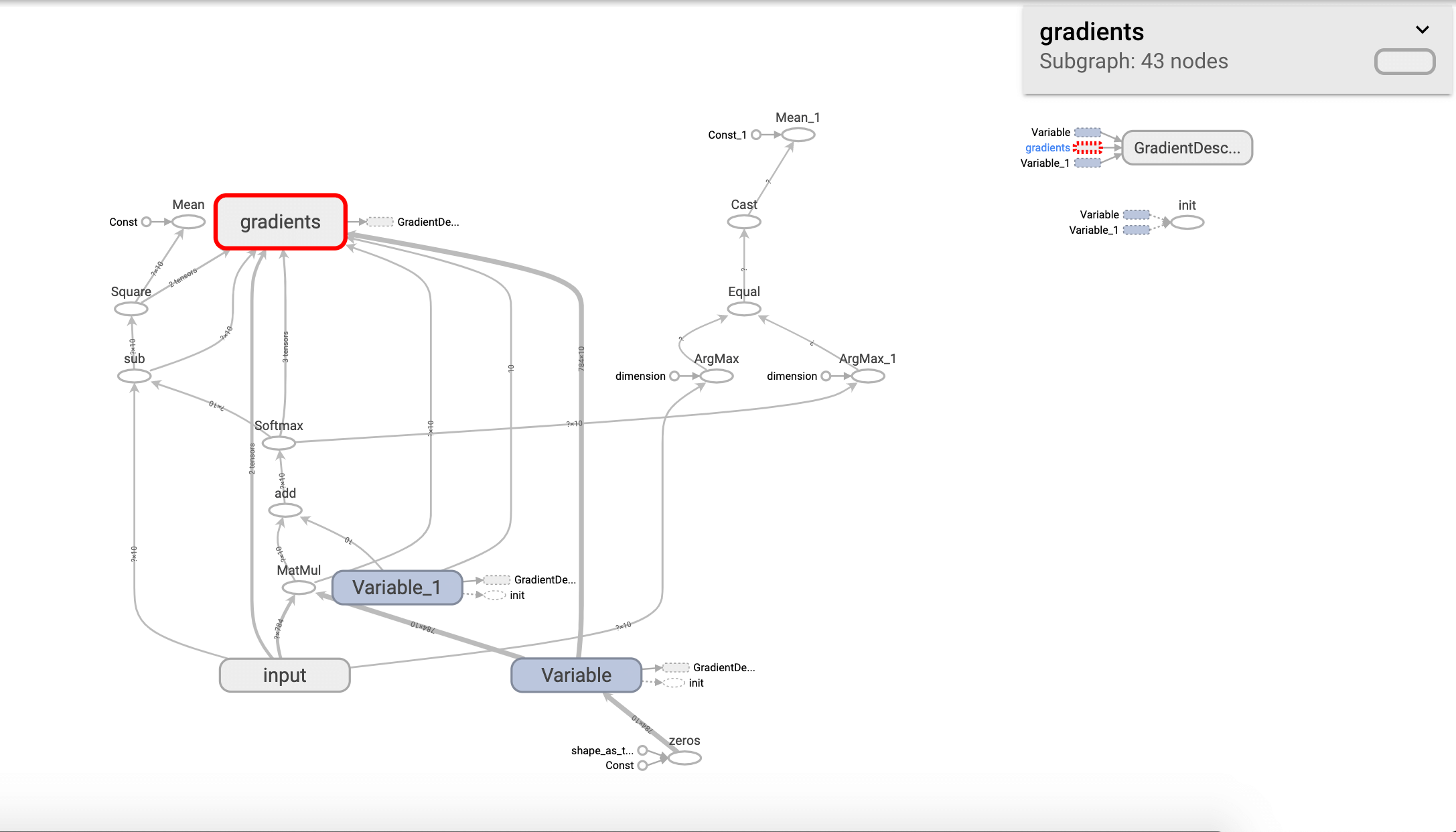
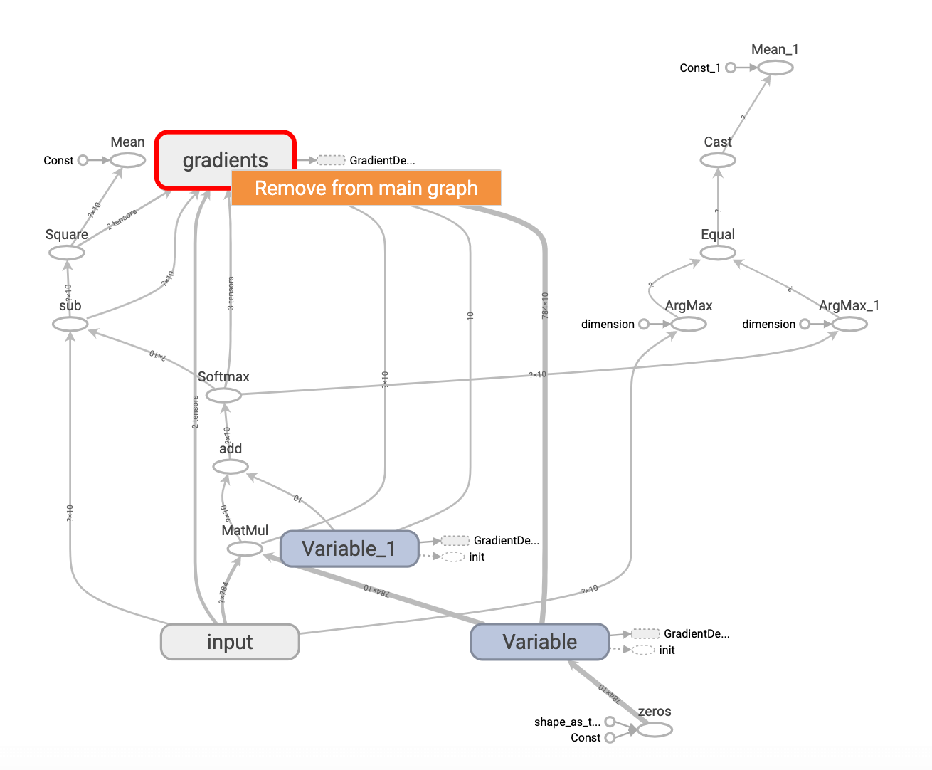
同理,我们也可以将其从主图移除:
对网络的输出层进行如下改动,重新生成log文件:
1
2
3
4
5
6
7
8
9
10
with tf.name_scope("layer"):
    #创建一个简单的神经网络(无隐藏层)
    with tf.name_scope("weights"):
        W=tf.Variable(tf.zeros([784,10]),name="W")
    with tf.name_scope("biases"):
        b=tf.Variable(tf.zeros([10]),name="b")
    with tf.name_scope("wx_plus_b"):
        wx_plus_b=tf.matmul(x,W)+b
    with tf.name_scope("softmax"):
        prediction=tf.nn.softmax(wx_plus_b)
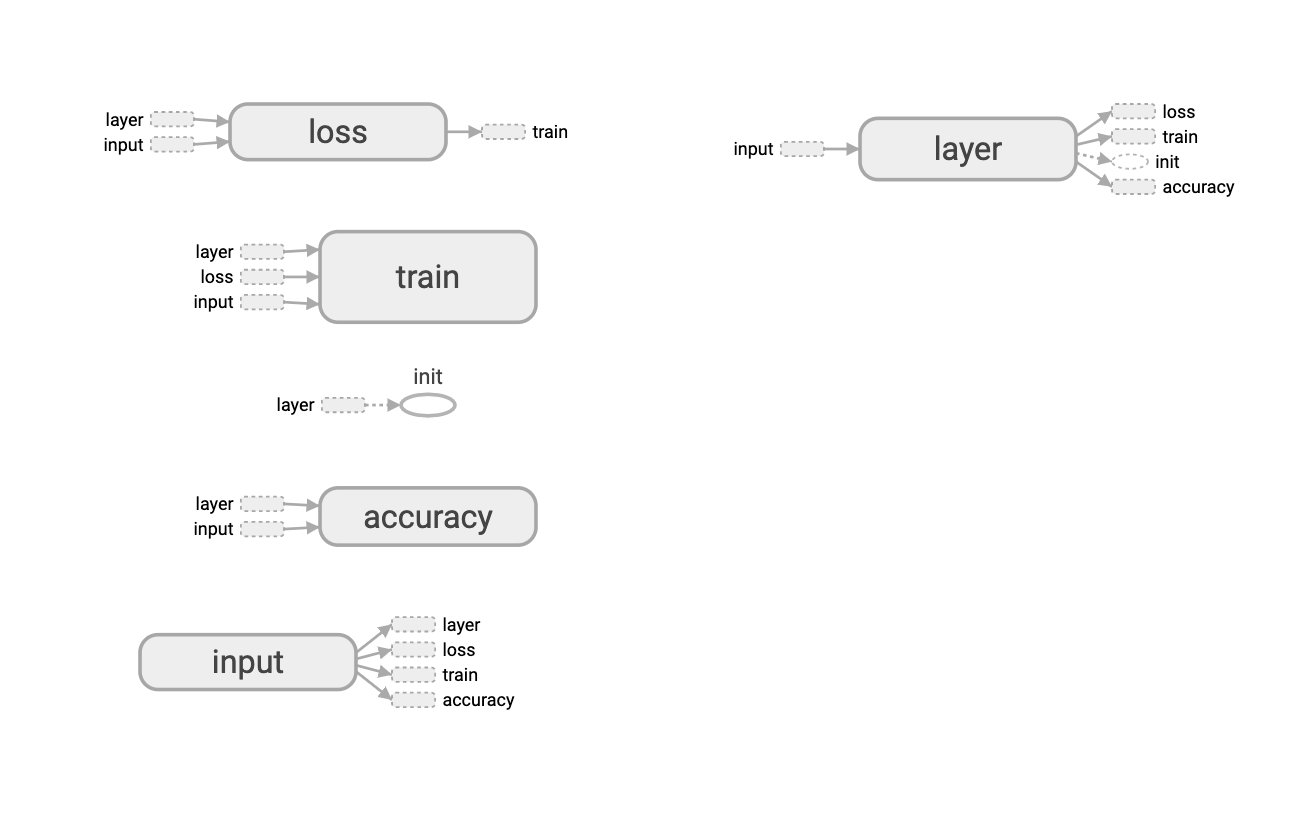
graph中输出层结构的变化:
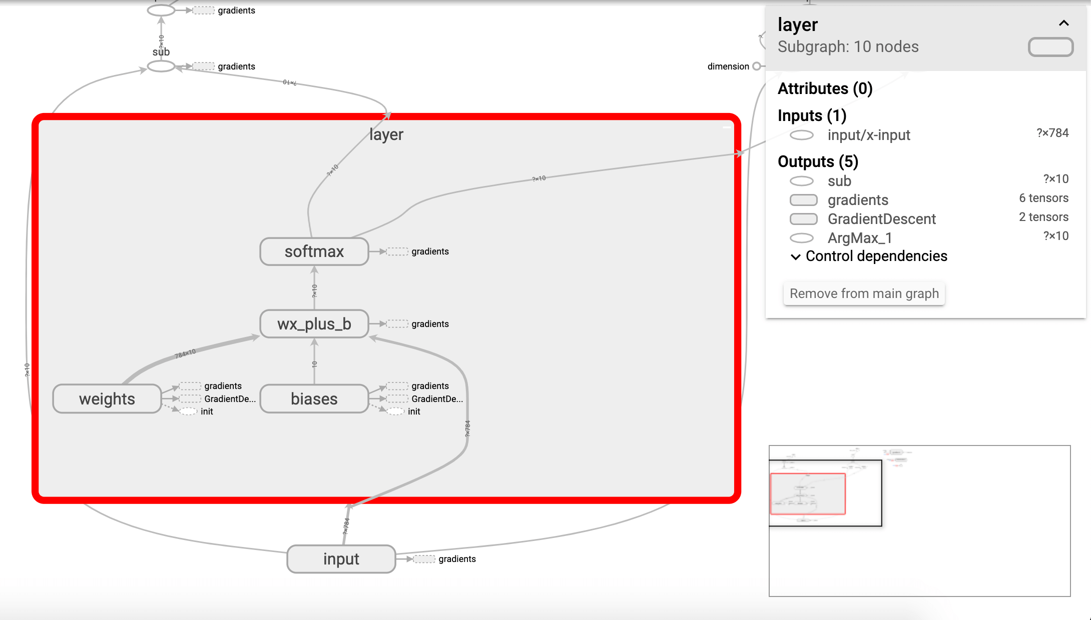
可以双击任意命名空间查看更加详细的信息,例如:
将程序中的其他部分也添加命名空间:
1
2
3
4
5
6
7
8
9
10
11
12
13
14
15
16
with tf.name_scope("loss"):
    #均方误差
    loss=tf.reduce_mean(tf.square(y-prediction))
with tf.name_scope("train"):
    #梯度下降法
    train_step=tf.train.GradientDescentOptimizer(0.2).minimize(loss)

#初始化变量
init=tf.global_variables_initializer()#有默认的init命名空间,不再额外定义命名空间

with tf.name_scope("accuracy"):
    #统计预测结果
    with tf.name_scope("correct_prediction"):
        correct_prediction=tf.equal(tf.argmax(y,1),tf.argmax(prediction,1))#返回一个布尔型的列表
    with tf.name_scope("accuracy"):
        accuracy=tf.reduce_mean(tf.cast(correct_prediction,tf.float32))
重新生成log文件并加载graph:
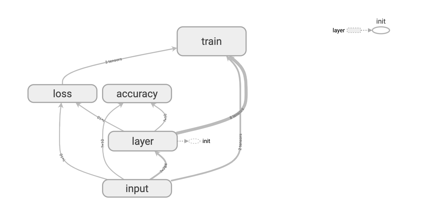
将网络的各个部分定义命名空间之后,网络图明显简单易懂了许多。
可以把所有命名空间都从主图移除:
2.2.SCALARS
tf.summary.scalar用来显示标量信息。一般在画loss,accuracy时会用到这个函数。例如,在2.1部分代码的基础上主要添加以下函数:
1
2
3
4
5
6
7
8
9
#省略
with tf.name_scope("loss"):
    #均方误差
    loss=tf.reduce_mean(tf.square(y-prediction))
    tf.summary.scalar('loss',loss)
#省略
    with tf.name_scope("accuracy"):
        accuracy=tf.reduce_mean(tf.cast(correct_prediction,tf.float32))
        tf.summary.scalar('accuracy',accuracy)
完整的代码请见:链接。
进入tensorboard的界面,点击SCALARS,可以看到accuracy随着epoch的变化:
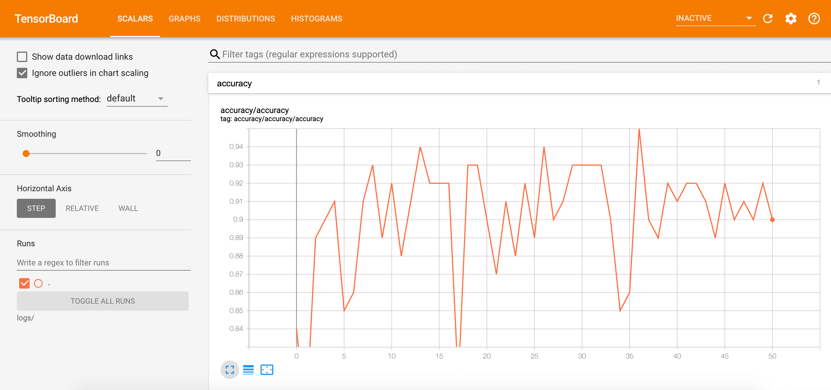
通过调节左侧的Smoothing使曲线变得平滑:
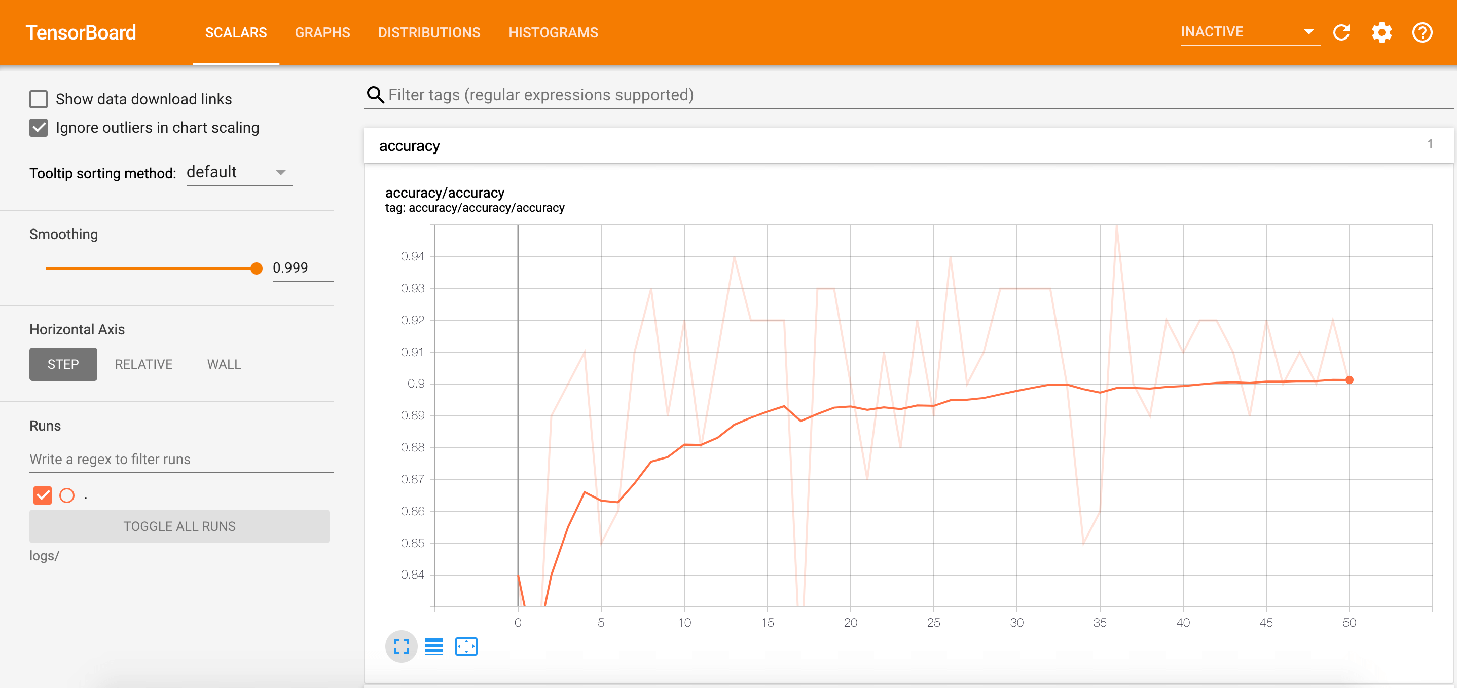
上图背景中被虚化的曲线为未平滑时的曲线。
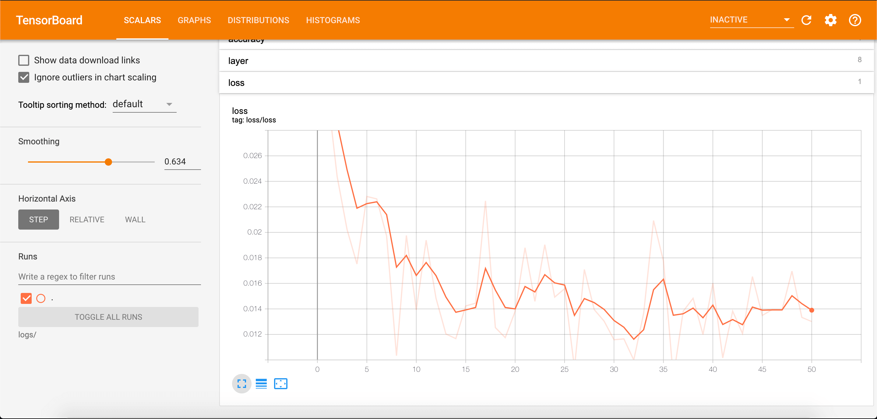
同样的,我们也可以查看loss随着epoch的变化:
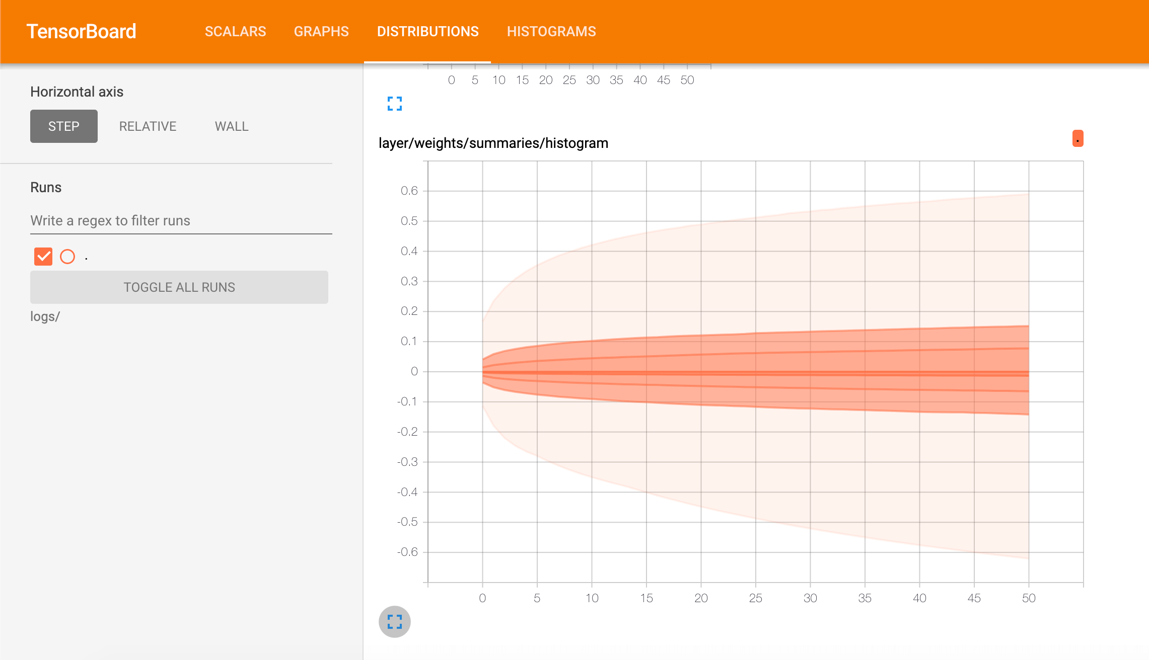
2.3.DISTRIBUTIONS和HISTOGRAMS
HISTOGRAMS和DISTRIBUTIONS这两种图的数据源是相同的,只是从不同的视角、以不同的方式来表示数据的分布情况。
使用以下语句:
1
tf.summary.histogram('histogram',var)#直方图
例如我们通过DISTRIBUTIONS查看weights的变化:
通过HISTOGRAMS查看weights的变化:
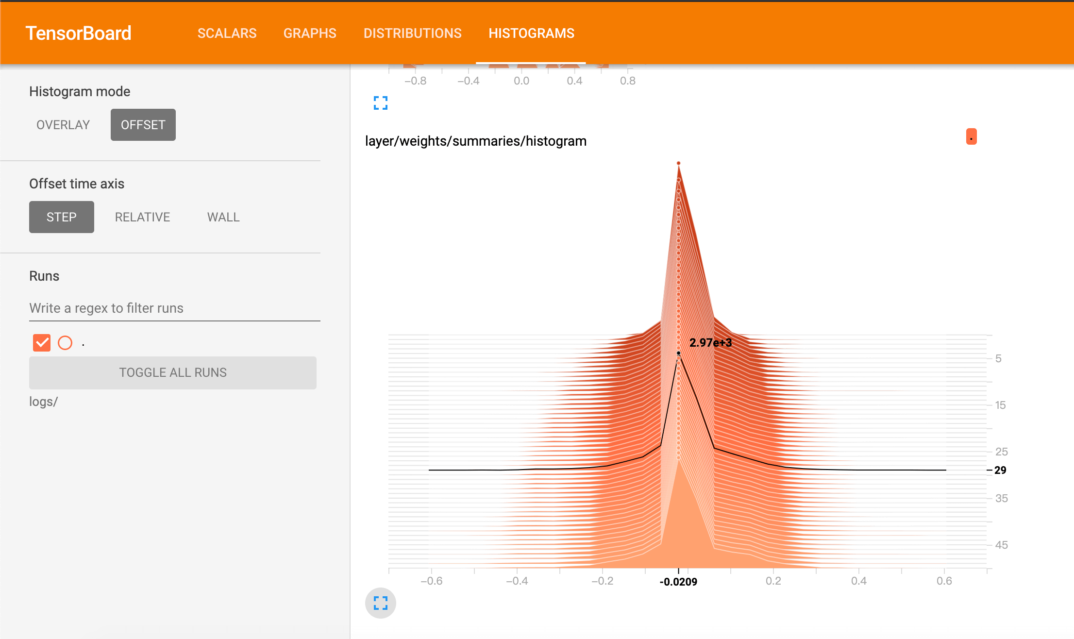
鼠标悬停在不同的epoch上,可以查看该epoch下,weights的分布情况。
3.TensorBoard可视化
TensorBoard提供了一个内置的交互式可视化工具:Embedding Projector。该功能用于在二维或三维空间对高维数据进行探索。
完整代码见:TensorBoard可视化。
关于代码中一些内容的解释:
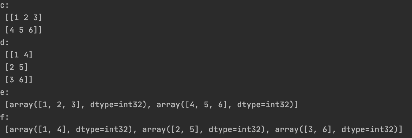
👉embedding = tf.Variable(tf.stack(mnist.test.images[:image_num]), trainable=False, name='embedding')
✓tf.stack()和tf.unstack():
tf.stack()是一个矩阵拼接的函数。tf.unstack()是一个矩阵分解的函数。
1
2
3
4
5
6
7
8
9
10
11
12
import tensorflow as tf
a=tf.constant([1,2,3])
b=tf.constant([4,5,6])
c=tf.stack([a,b],axis=0)
d=tf.stack([a,b],axis=1)
e=tf.unstack(c,axis=0)
f=tf.unstack(c,axis=1)
with tf.Session() as sess:
	print("c:\n",sess.run(c))
	print("d:\n",sess.run(d))
	print("e:\n",sess.run(e))
	print("f:\n",sess.run(f))
✓mnist.test.images[:image_num]表示前image_num张测试图片。
✓trainable=False时,该变量不会被优化器更新,即无法更改。可用于定义训练过程中不用或不能被更新的参数。
👉image_shaped_input = tf.reshape(x, [-1, 28, 28, 1])
✓tf.reshape(tensor, shape, name=None)。其中shape为一个列表形式,特殊的一点是列表中可以存在-1。-1代表的含义是不用我们自己指定这一维的大小,函数会自动计算,但列表中只能存在一个-1。(当然如果存在多个-1,就是一个存在多解的方程了)。
👉tf.summary.image('input', image_shaped_input, 10)
✓tf.summary.image(name, tensor, max_outputs=3, collections=None, family=None)输出Summary带有图像的协议缓冲区。构建图像的tensor必须是4维的:[batch_size, height, width, channels]。
👉tf.gfile:
tf.gfile.Exists(filename):判断目录或文件是否存在,filename可为目录路径或带文件名的路径,有该目录则返回True,否则False。tf.gfile.DeleteRecursively(dirname):递归删除所有目录及其文件,dirname即目录名,无返回。
👉保存模型:
1
2
saver = tf.train.Saver()
saver.save(sess, DIR + 'projector/projector/a_model.ckpt', global_step=max_steps)
👉可视化部分核心代码:
1
2
3
4
5
6
7
config = projector.ProjectorConfig()
embed = config.embeddings.add()
embed.tensor_name = embedding.name
embed.metadata_path = DIR + 'projector/projector/metadata.tsv'
embed.sprite.image_path = DIR + 'projector/data/mnist_10k_sprite.png'
embed.sprite.single_image_dim.extend([28, 28])
projector.visualize_embeddings(projector_writer, config)
👉tf.RunOptions()和tf.RunMetadata():用于收集网络运行过程中的跟踪信息,包括延时,内存开销等。
成功运行代码之后,可以发现projector文件夹下生成了很多文件:
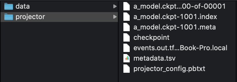
打开终端,输入(改为自己的路径):
1
tensorboard --logdir=projector/projector/
按照命令给的网址打开tensorboard。
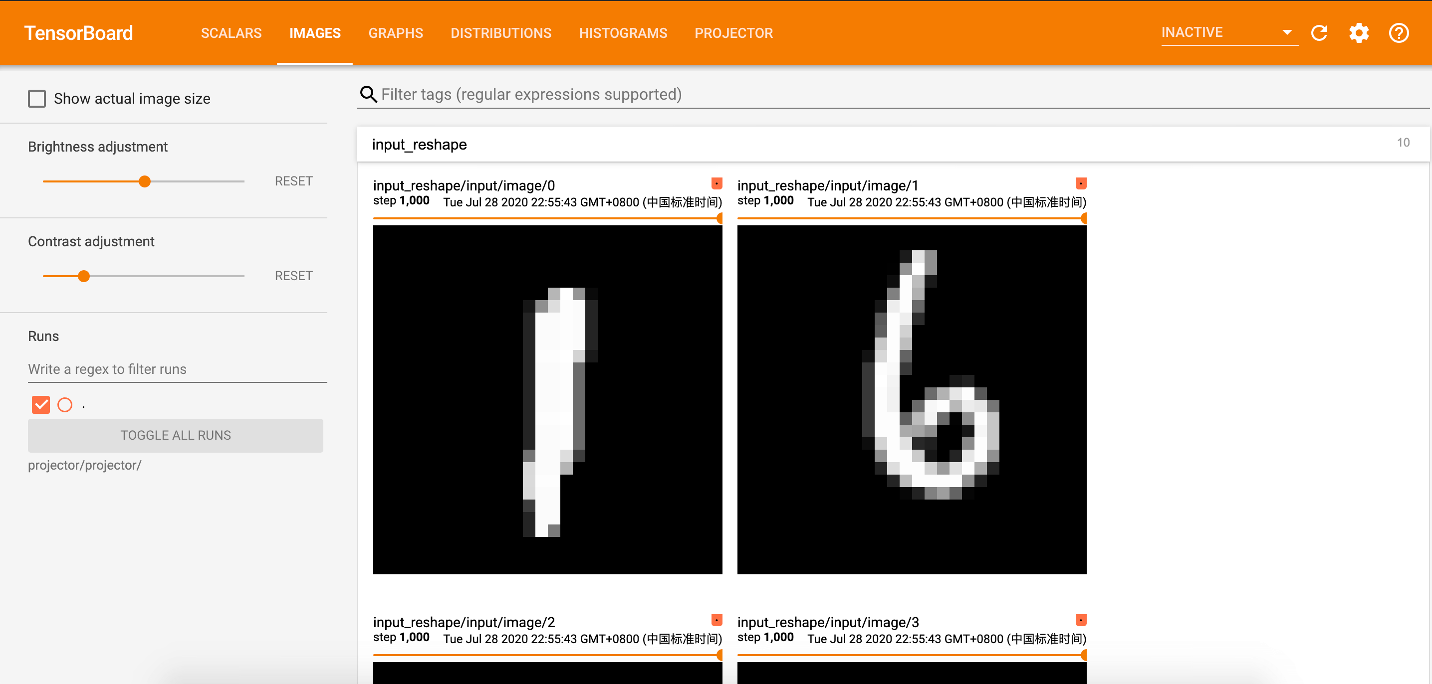
3.1.IMAGES
我们在代码中定义了tf.summary.image():
1
2
3
4
# 显示图片
with tf.name_scope('input_reshape'):
    image_shaped_input = tf.reshape(x, [-1, 28, 28, 1])
    tf.summary.image('input', image_shaped_input, 10)
在tensorboard中显示的结果:
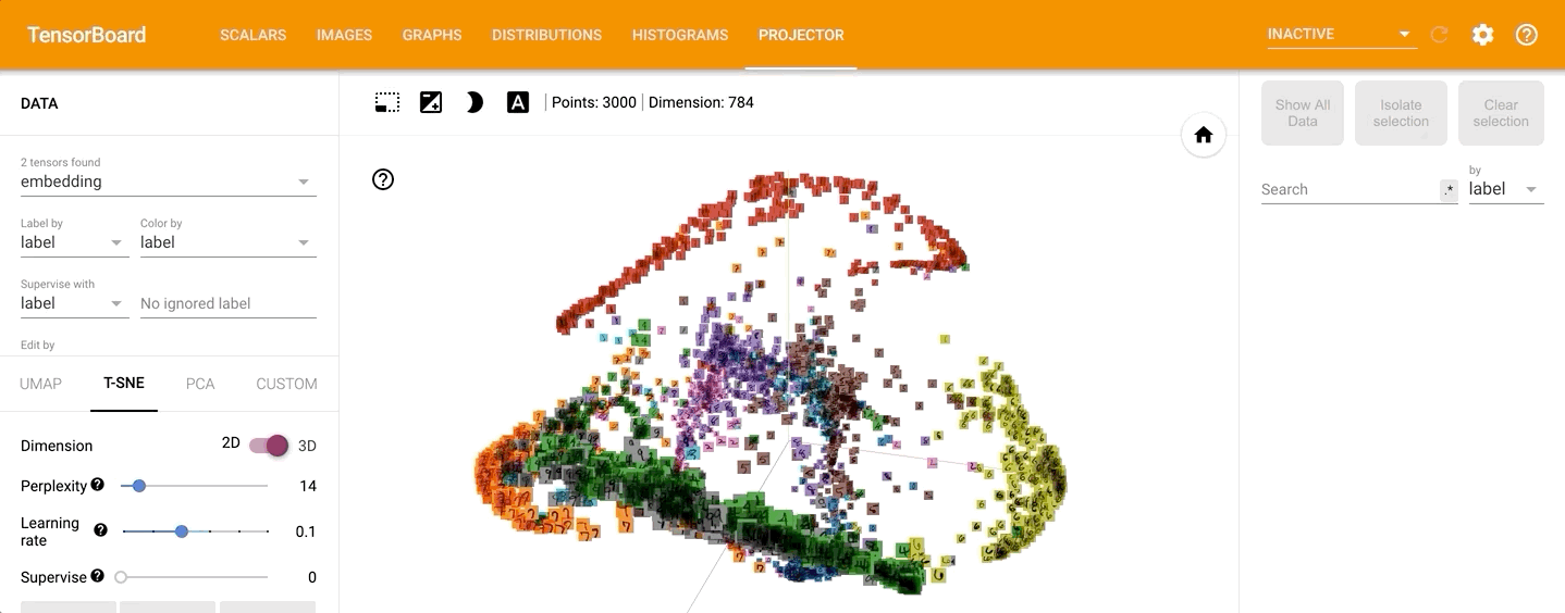
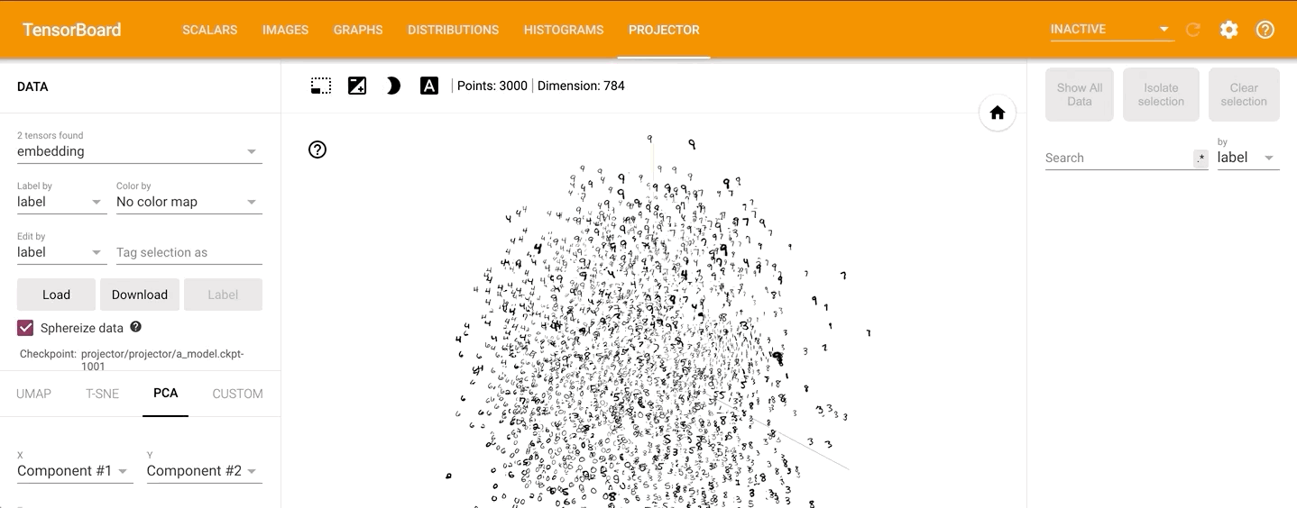
3.2.PROJECTOR
如果点击
PROJECTOR,出现如下错误:”projector/projector/../Demo5/projector/projector/metadata.tsv” not found, or is not a file。解决办法为打开projector文件夹下的projector_config.pbtxt,把里面的metadata_path和image_path改为绝对路径即可。
点击PROJECTOR,可以看到数据的原始分布见如下动图:
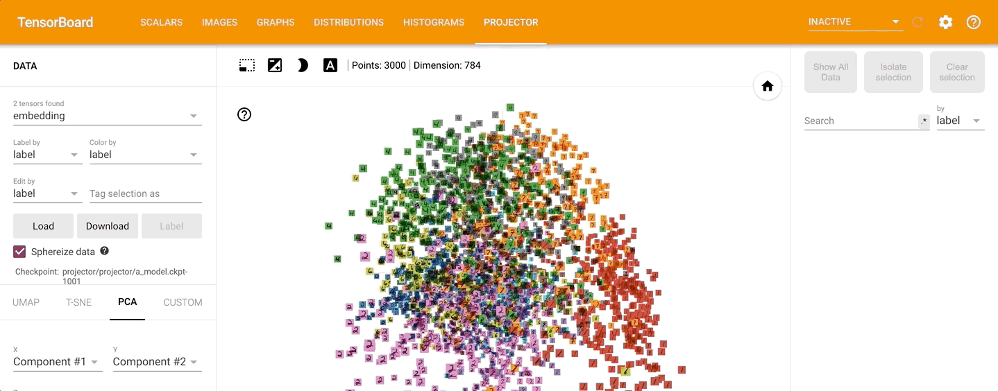
通过左侧的“Color by”可以将不同的数字标识为不同的颜色:
点击左侧的“T-SNE”,可以直观的观察其训练过程,并且可以调整不同的学习率: