【机器学习基础】系列博客为参考周志华老师的《机器学习》一书,自己所做的读书笔记。
本文为原创文章,未经本人允许,禁止转载。转载请注明出处。
1.密度聚类
密度聚类亦称“基于密度的聚类”(density-based clustering),此类算法假设聚类结构能通过样本分布的紧密程度确定。通常情形下,密度聚类算法从样本密度的角度来考察样本之间的可连接性,并基于可连接样本不断扩展聚类簇以获得最终的聚类结果。
DBSCAN是一种著名的密度聚类算法,它基于一组“邻域”(neighborhood)参数$(\epsilon, MinPts)$来刻画样本分布的紧密程度。给定数据集$D=\{\mathbf{x}_1,\mathbf{x}_2,…,\mathbf{x}_m \}$,定义下面这几个概念:
DBSCAN全称“Density-Based Spatial Clustering of Applications with Noise”。
- $\epsilon-$邻域:对$\mathbf{x}_j \in D$,其$\epsilon-$邻域包含样本集$D$中与$\mathbf{x}_j$的距离不大于$\epsilon$的样本,即$N_{\epsilon}(\mathbf{x}_j)= \{ \mathbf{x}_i \in D \mid \text{dist} (\mathbf{x}_i,\mathbf{x}_j) \leqslant \epsilon\}$;
- 核心对象(core object):若$\mathbf{x}_j$的$\epsilon-$邻域至少包含$MinPts$个样本,即$\lvert N_{\epsilon}(\mathbf{x}_j) \rvert \geqslant MinPts$,则$\mathbf{x}_j$是一个核心对象。
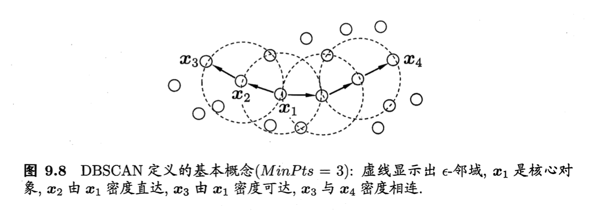
- 密度直达(directly density-reachable):若$\mathbf{x}_j$位于$\mathbf{x}_i$的$\epsilon-$邻域中,且$\mathbf{x}_i$是核心对象,则称$\mathbf{x}_j$由$\mathbf{x}_i$密度直达;
- 密度可达(density-reachable):对$\mathbf{x}_i$与$\mathbf{x}_j$,若存在样本序列$\mathbf{p}_1,\mathbf{p}_2,…,\mathbf{p}_n$,其中$\mathbf{p}_1=\mathbf{x}_i,\mathbf{p}_n=\mathbf{x}_j$且$\mathbf{p}_{i+1}$由$\mathbf{p}_i$密度直达,则称$\mathbf{x}_j$由$\mathbf{x}_i$密度可达;
- 密度相连(density-connected):对$\mathbf{x}_i$与$\mathbf{x}_j$,若存在$\mathbf{x}_k$使得$\mathbf{x}_i$与$\mathbf{x}_j$均由$\mathbf{x}_k$密度可达,则称$\mathbf{x}_i$与$\mathbf{x}_j$密度相连。
距离函数$\text{dist} (\cdot , \cdot)$默认为欧氏距离。
密度直达关系通常不满足对称性。
密度可达关系满足直递性,但不满足对称性。
密度相连关系满足对称性。
上述概念的直观显示:
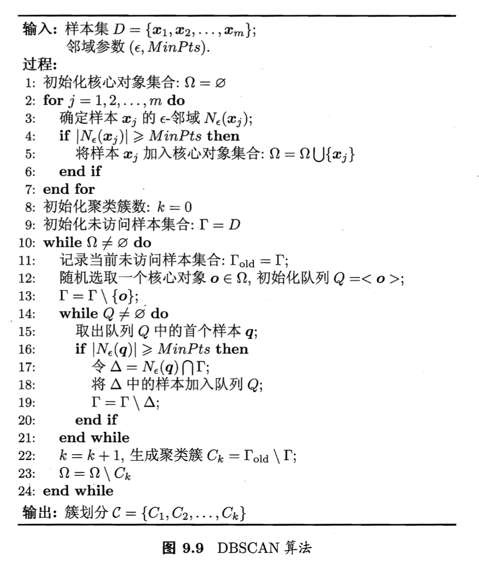
DBSCAN算法的流程见下:
以以下数据集为例:
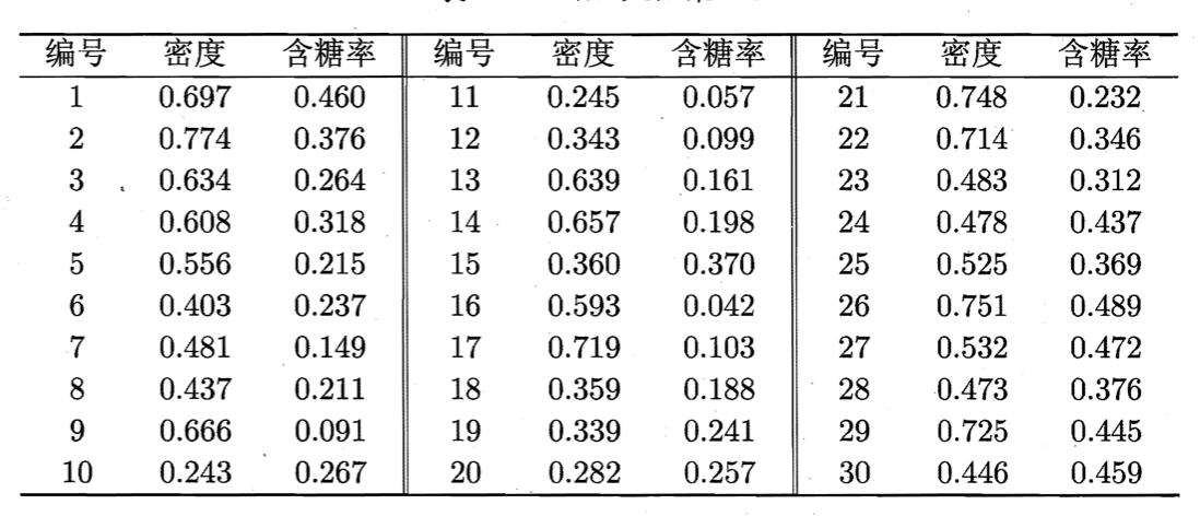
假定邻域参数$(\epsilon, MinPts)$设置为$\epsilon=0.11,MinPts=5$。DBSCAN算法先找出各样本的$\epsilon-$邻域并确定核心对象集合:$\Omega= \{ \mathbf{x}_3,\mathbf{x}_5,\mathbf{x}_6,\mathbf{x}_8,\mathbf{x}_9,\mathbf{x}_{13},\mathbf{x}_{14},\mathbf{x}_{18},\mathbf{x}_{19},\mathbf{x}_{24},\mathbf{x}_{25},\mathbf{x}_{28},\mathbf{x}_{29} \}$。然后,从$\Omega$中随机选取一个核心对象作为种子,找出由它密度可达的所有样本,这就构成了第一个聚类簇。不失一般性,假定核心对象$\mathbf{x}_8$被选中作为种子,则DBSCAN生成的第一个聚类簇为:
\[C_1= \{\mathbf{x}_6,\mathbf{x}_7,\mathbf{x}_8,\mathbf{x}_{10},\mathbf{x}_{12},\mathbf{x}_{18},\mathbf{x}_{19},\mathbf{x}_{20},\mathbf{x}_{23} \}\]然后,DBSCAN将$C_1$中包含的核心对象从$\Omega$中去除:$\Omega = \Omega \setminus C_1=\{\mathbf{x}_3,\mathbf{x}_5,\mathbf{x}_9,\mathbf{x}_{13},\mathbf{x}_{14},\mathbf{x}_{24},\mathbf{x}_{25},\mathbf{x}_{28},\mathbf{x}_{29} \}$。再从更新后的集合$\Omega$中随机选取一个核心对象作为种子来生成下一个聚类簇。上述过程不断重复,直至$\Omega$为空。下图显示出DBSCAN先后生成聚类簇的情况:
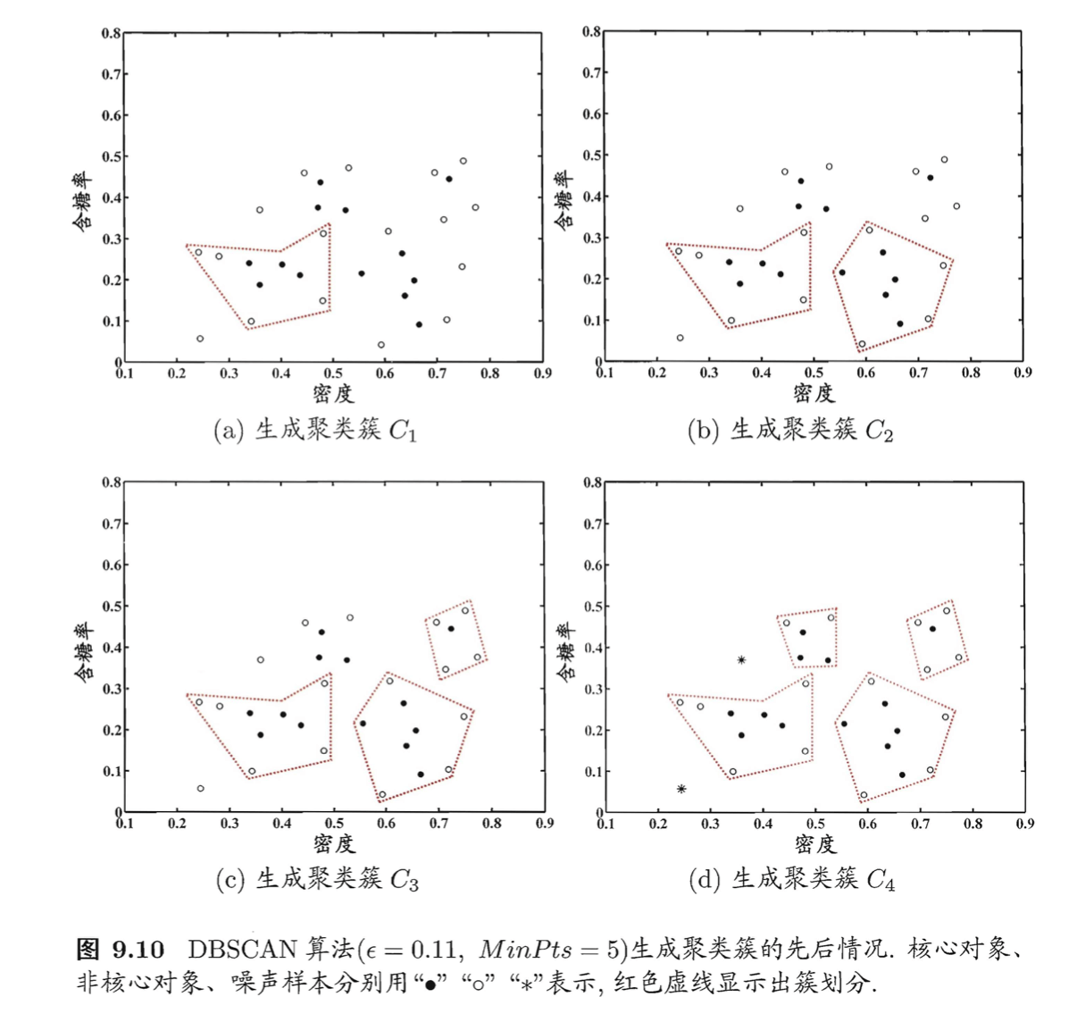
$C_1$之后生成的聚类簇为:
\[C_2= \{ \mathbf{x}_3,\mathbf{x}_4,\mathbf{x}_5,\mathbf{x}_9,\mathbf{x}_{13},\mathbf{x}_{14},\mathbf{x}_{16},\mathbf{x}_{17},\mathbf{x}_{21} \}\] \[C_3=\{\mathbf{x}_1,\mathbf{x}_2,\mathbf{x}_{22},\mathbf{x}_{26},\mathbf{x}_{29} \}\] \[C_4=\{ \mathbf{x}_{24},\mathbf{x}_{25},\mathbf{x}_{27},\mathbf{x}_{28},\mathbf{x}_{30} \}\]