本文为原创文章，未经本人允许，禁止转载。转载请注明出处。

1.Word2Vec

Word2Vec相关知识请见：【深度学习基础】第四十五课：自然语言处理与词嵌入。

2.代码实现

👉载入包：

import collections
import math
import os
import random
import zipfile

import numpy as np
from six.moves import urllib
from six.moves import xrange  # pylint: disable=redefined-builtin
import tensorflow as tf

👉下载数据集：

# Step 1: Download the data.
url = 'http://mattmahoney.net/dc/'

# 下载数据集
def maybe_download(filename, expected_bytes):
    """Download a file if not present, and make sure it's the right size."""
    if not os.path.exists(filename):
        filename, _ = urllib.request.urlretrieve(url + filename, filename)
    # 获取文件相关属性
    statinfo = os.stat(filename)
    # 比对文件的大小是否正确
    if statinfo.st_size == expected_bytes:
        print('Found and verified', filename)
    else:
        print(statinfo.st_size)
        raise Exception(
            'Failed to verify ' + filename + '. Can you get to it with a browser?')
    return filename

filename = maybe_download('text8.zip', 31344016)

os.path.exists()用于判断文件是否存在，如果存在则返回true；如果不存在，则返回false。

urllib.request.urlretrieve(url,filename)用于将url（可以是本地路径也可以是网络链接）表示的对象复制到filename（保存到本地的路径）。

os.stat(path)用于在给定的路径上执行一个系统stat的调用。返回值：

st_mode：inode保护模式。
st_ino：inode节点号。
st_dev：inode驻留的设备。
st_nlink：inode的链接数。
st_uid：所有者的用户ID。
st_gid：所有者的组ID。
st_size：普通文件以字节为单位的大小；包含等待某些特殊文件的数据。
st_atime：上次访问的时间。
st_mtime：最后一次修改的时间。
st_ctime：由操作系统报告的“ctime”。在某些系统上（如Unix）是最新的元数据更改的时间，在其它系统上（如Windows）是创建时间（详细信息参见平台的文档）。

👉读取数据：

# Read the data into a list of strings.
def read_data(filename):
    """Extract the first file enclosed in a zip file as a list of words"""
    with zipfile.ZipFile(filename) as f:
        data = tf.compat.as_str(f.read(f.namelist()[0])).split()
    return data

# 单词表
words = read_data(filename)

zipfile.ZipFile(file,mode)：如果mode=’r’，则为读取压缩文件file中的内容；如果mode=’w’，则为向压缩文件file中写入内容。

ZipFile.namelist()：获取压缩文件内所有文件的名称列表。

tf.compat.as_str：将目标转化为字符串格式。

👉创建一个单词表（共50000个最常见的单词，包含UNK）：

# Step 2: Build the dictionary and replace rare words with UNK token.
# 只留50000个单词，其他的词都归为UNK
vocabulary_size = 50000

def build_dataset(words, vocabulary_size):
    count = [['UNK', -1]]
    count.extend(collections.Counter(words).most_common(vocabulary_size - 1))
    # 生成 dictionary，词对应编号, word:id(0-49999)
    # 词频越高编号越小
    dictionary = dict()
    for word, _ in count:
        dictionary[word] = len(dictionary)
    # data把数据集的词都编号
    data = list()
    unk_count = 0
    for word in words:
        if word in dictionary:
            index = dictionary[word]
        else:
            index = 0  # dictionary['UNK']
            unk_count += 1
        data.append(index)
    # 记录UNK词的数量
    count[0][1] = unk_count
    # 编号对应词的字典
    reverse_dictionary = dict(zip(dictionary.values(), dictionary.keys()))
    return data, count, dictionary, reverse_dictionary

# data 数据集，编号形式
# count 前50000个出现次数最多的词
# dictionary 词对应编号
# reverse_dictionary 编号对应词
data, count, dictionary, reverse_dictionary = build_dataset(words, vocabulary_size)
del words  # Hint to reduce memory.

👉产生batch：

data_index = 0

# Step 3: Function to generate a training batch for the skip-gram model.
def generate_batch(batch_size, num_skips, skip_window):
    global data_index
    assert batch_size % num_skips == 0
    assert num_skips <= 2 * skip_window

    batch = np.ndarray(shape=(batch_size), dtype=np.int32)
    labels = np.ndarray(shape=(batch_size, 1), dtype=np.int32)

    span = 2 * skip_window + 1  # [ skip_window target skip_window ]
    buffer = collections.deque(maxlen=span)

    # 循环3次
    for _ in range(span):
        buffer.append(data[data_index])
        data_index = (data_index + 1) % len(data)
    # 获取batch和labels
    for i in range(batch_size // num_skips):
        target = skip_window  # target label at the center of the buffer
        targets_to_avoid = [skip_window]
        # 循环2次，一个目标单词对应两个上下文单词
        for j in range(num_skips):
            while target in targets_to_avoid:
                # 可能先拿到前面的单词也可能先拿到后面的单词
                target = random.randint(0, span - 1)
            targets_to_avoid.append(target)
            batch[i * num_skips + j] = buffer[skip_window]
            labels[i * num_skips + j, 0] = buffer[target]
        buffer.append(data[data_index])
        data_index = (data_index + 1) % len(data)
    # Backtrack a little bit to avoid skipping words in the end of a batch
    # 回溯3个词。因为执行完一个batch的操作之后，data_index会往右多偏移span个位置
    data_index = (data_index + len(data) - span) % len(data)
    return batch, labels

# 打印sample data
batch, labels = generate_batch(batch_size=8, num_skips=2, skip_window=1)

举个例子解释一下，数据集中前6个单词在单词表中的索引见下：

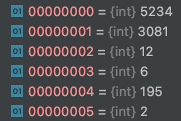
如果以第1个单词（3081）为中心，则其上下文为第0个单词（5234）和第2个单词（12）；如果以第2个单词（12）为中心，则其上下文为第1个单词（3081）和第3个单词（6）；剩余以此类推，则此时generate_batch函数返回的batch为：

[3081 3081 12 12 6 6 195 195]

返回的labels为：

[
[5234]
[12]
[3081]
[6]
[12]
[195]
[6]
[2]
]

对应关系为：

originated -> 5234 anarchism
originated -> 12 as
as -> 3081 originated
as -> 6 a
a -> 12 as
a -> 195 term
term -> 6 a
term -> 2 of

collections.deque用于产生一个双向队列，可以从两端append、extend或pop：

import collections
d = collections.deque([])
d.append('a') # 在最右边添加一个元素，此时 d=deque('a')
d.appendleft('b') # 在最左边添加一个元素，此时 d=deque(['b', 'a'])
d.extend(['c','d']) # 在最右边添加所有元素，此时 d=deque(['b', 'a', 'c', 'd'])
d.extendleft(['e','f']) # 在最左边添加所有元素，此时 d=deque(['f', 'e', 'b', 'a', 'c', 'd'])
d.pop() # 将最右边的元素取出，返回 'd'，此时 d=deque(['f', 'e', 'b', 'a', 'c'])
d.popleft() # 将最左边的元素取出，返回 'f'，此时 d=deque(['e', 'b', 'a', 'c'])
d.rotate(-2) # 向左旋转两个位置（正数则向右旋转），此时 d=deque(['a', 'c', 'e', 'b'])
d.count('a') # 队列中'a'的个数，返回 1
d.remove('c') # 从队列中将'c'删除，此时 d=deque(['a', 'e', 'b'])
d.reverse() # 将队列倒序，此时 d=deque(['b', 'e', 'a'])
f=d.copy()
print(f)#deque(['b', 'e', 'a'])
f.clear()
print(f)#deque([])
 
#可以指定队列的长度，如果添加的元素超过指定长度，则原元素会被挤出。
e=collections.deque(maxlen=5)
e.extend([1,2,3,4,5])
e.append("a")
print(e)
#deque([2, 3, 4, 5, 'a'], maxlen=5)
e.appendleft("b")
print(e)
#deque(['b', 2, 3, 4, 5], maxlen=5)
e.extendleft(["c","d"])
print(e)
#deque(['d', 'c', 'b', 2, 3], maxlen=5)

random.randint(a,b)：参数a和参数b必须是整数，该函数返回参数a和参数b之间的任意整数（$[a,b]$）。

👉建立skip-gram模型：

# Step 4: Build and train a skip-gram model.
batch_size = 128
embedding_size = 128  # Dimension of the embedding vector.
skip_window = 1  # How many words to consider left and right.
num_skips = 2  # How many times to reuse an input to generate a label.

# We pick a random validation set to sample nearest neighbors. Here we limit the
# validation samples to the words that have a low numeric ID, which by
# construction are also the most frequent.
valid_size = 16  # Random set of words to evaluate similarity on.
valid_window = 100  # Only pick dev samples in the head of the distribution.
# 从0-100抽取16个整数，无放回抽样
valid_examples = np.random.choice(valid_window, valid_size, replace=False)
# 负采样样本数
num_sampled = 64  # Number of negative examples to sample.

graph = tf.Graph()
with graph.as_default():
    # Input data.
    train_inputs = tf.placeholder(tf.int32, shape=[batch_size])
    train_labels = tf.placeholder(tf.int32, shape=[batch_size, 1])
    valid_dataset = tf.constant(valid_examples, dtype=tf.int32)

    # 词向量
    # Look up embeddings for inputs.
    embeddings = tf.Variable(
        tf.random_uniform([vocabulary_size, embedding_size], -1.0, 1.0))
    # embedding_lookup(params,ids)其实就是按照ids顺序返回params中的第ids行
    # 比如说，ids=[1,7,4],就是返回params中第1,7,4行。返回结果为由params的1,7,4行组成的tensor
    # 提取要训练的词
    embed = tf.nn.embedding_lookup(embeddings, train_inputs)

    # Construct the variables for the noise-contrastive estimation(NCE) loss
    nce_weights = tf.Variable(
        tf.truncated_normal([vocabulary_size, embedding_size],
                            stddev=1.0 / math.sqrt(embedding_size)))
    nce_biases = tf.Variable(tf.zeros([vocabulary_size]))

    # Compute the average NCE loss for the batch.
    # tf.nce_loss automatically draws a new sample of the negative labels each
    # time we evaluate the loss.
    loss = tf.reduce_mean(
        tf.nn.nce_loss(weights=nce_weights,
                       biases=nce_biases,
                       labels=train_labels,
                       inputs=embed,
                       num_sampled=num_sampled,
                       num_classes=vocabulary_size))

    # Construct the SGD optimizer using a learning rate of 1.0.
    optimizer = tf.train.GradientDescentOptimizer(1).minimize(loss)

    # Compute the cosine similarity between minibatch examples and all embeddings.
    norm = tf.sqrt(tf.reduce_sum(tf.square(embeddings), 1, keep_dims=True))
    normalized_embeddings = embeddings / norm
    # 抽取一些常用词来测试余弦相似度
    # valid_embeddings维度[16,128]
    valid_embeddings = tf.nn.embedding_lookup(
        normalized_embeddings, valid_dataset)
    # valid_size == 16
    # [16,128] * [128,50000] = [16,50000]
    # 16个词分别与50000个单词中的每一个计算内积
    similarity = tf.matmul(
        valid_embeddings, normalized_embeddings, transpose_b=True)

    # Add variable initializer.
    init = tf.global_variables_initializer()

numpy.random.choice(a, size=None, replace=True, p=None)用于生成随机样本，参数详解：

a：一维数组或者一个int型整数。如果a为数组，则从数组中的元素进行随机采样；如果a为int型整数，则采样范围为np.arange(a)。
size：随机采样的样本的数量。
replace：True表示有放回采样；False表示无放回采样。
p：与数组a对应，为a中每个元素被采样的概率。

tf.random_uniform(shape,
                  minval=0,
                  maxval=None,
                  dtype=dtypes.float32,
                  seed=None,
                  name=None)

用于产生[minval,maxval)范围内服从均匀分布的值。

tf.nn.embedding_lookup的作用见上述代码注释。

tf.nn.nce_loss：如果使用softmax函数，则类别数太多，导致计算量太大，所以这里使用NCE loss（原文：Noise-contrastive estimation: A new estimation principle for unnormalized statistical models），将多分类问题转化成二分类。

余弦相似度：

\[similarity = \cos (\theta) = \frac{A \cdot B}{\parallel A \parallel \parallel B \parallel }\]

参照内积的计算。

👉训练模型：

# Step 5: Begin training.
num_steps = 100001
final_embeddings = []

with tf.Session(graph=graph) as session:
    # We must initialize all variables before we use them.
    init.run()
    print("Initialized")

    average_loss = 0
    for step in xrange(num_steps):
        # 获取一个批次的target，以及对应的labels，都是编号形式的
        batch_inputs, batch_labels = generate_batch(
            batch_size, num_skips, skip_window)
        feed_dict = {train_inputs: batch_inputs, train_labels: batch_labels}

        # We perform one update step by evaluating the optimizer op (including it
        # in the list of returned values for session.run()
        _, loss_val = session.run([optimizer, loss], feed_dict=feed_dict)
        average_loss += loss_val

        # 计算训练2000次的平均loss
        if step % 2000 == 0:
            if step > 0:
                average_loss /= 2000
            # The average loss is an estimate of the loss over the last 2000 batches.
            print("Average loss at step ", step, ": ", average_loss)
            average_loss = 0

        # Note that this is expensive (~20% slowdown if computed every 500 steps)
        if step % 20000 == 0:
            sim = similarity.eval()
            # 计算验证集的余弦相似度最高的词
            for i in xrange(valid_size):
                # 根据id拿到对应单词
                valid_word = reverse_dictionary[valid_examples[i]]
                top_k = 8  # number of nearest neighbors
                # 从大到小排序，排除自己本身，取前top_k个值
                nearest = (-sim[i, :]).argsort()[1:top_k + 1]
                log_str = "Nearest to %s:" % valid_word
                for k in xrange(top_k):
                    close_word = reverse_dictionary[nearest[k]]
                    log_str = "%s %s," % (log_str, close_word)
                print(log_str)
    # 训练结束得到的词向量
    final_embeddings = normalized_embeddings.eval()

xrange和range用法完全相同，所不同的是生成的不是一个数组，而是一个生成器。xrange已在python3中被取消，和range函数合并为range。

argsort将元素从小到大排序并返回其对应的索引：

import numpy as np
a=np.array([[3,2,5],[6,3,9]])
print(a[0,:]) #array([3, 2, 5])
print(-a[0,:]) #array([-3, -2, -5])
#最小值为-5，对应索引2
#第二小的值为-3，对应索引0
#最大值为-2，对应索引1
print((-a[0,:]).argsort()) #array([2, 0, 1])

👉使用TSNE进行降维可视化：

3.代码地址

Word2Vec

【Tensorflow基础】第十三课：Word2Vec

os.path.exists，urllib.request.urlretrieve，os.stat，zipfile.ZipFile，ZipFile.namelist，tf.compat.as_str，collections.deque，random.randint，numpy.random.choice，tf.nn.embedding_lookup，tf.nn.nce_loss，xrange，argsort，TSNE降维可视化，tf.random_uniform

1.Word2Vec

2.代码实现

3.代码地址

4.参考资料

CATALOG

FEATURED TAGS