【从零开始构建大语言模型】系列博客为”Build a Large Language Model (From Scratch)”一书的个人读书笔记。
- 原书链接:Build a Large Language Model (From Scratch)。
- 官方示例代码:LLMs-from-scratch。
本文为原创文章,未经本人允许,禁止转载。转载请注明出处。
1.Coding attention mechanisms
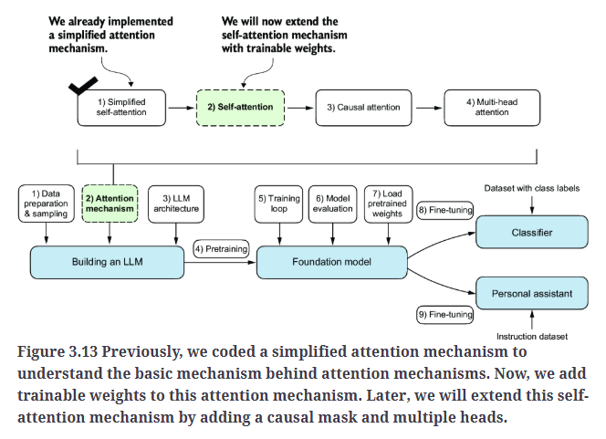
本博文将深入探讨LLM架构中的一个核心部分:注意力机制,如Fig3.1所示。
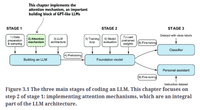
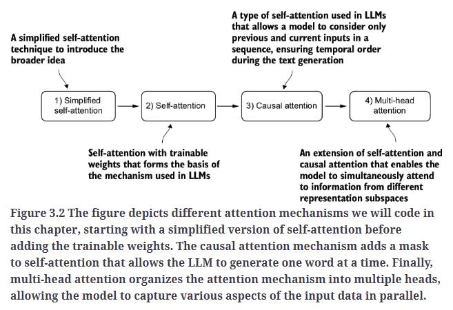
我们将实现四种不同的注意力机制变体,如Fig3.2所示。这些不同的注意力变体是在前一种基础上逐步构建的,目标是最终实现一种紧凑且高效的多头注意力(Multi-Head Attention)实现方案,然后将其集成到LLM架构中。
2.The problem with modeling long sequences
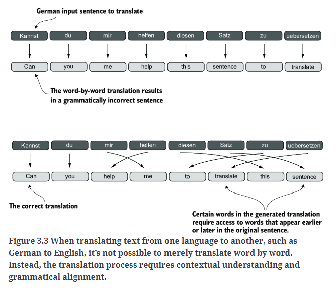
在深入探讨LLM核心的自注意力机制之前,让我们先思考在不使用注意力机制的传统架构中存在的问题。假设我们要开发一个语言翻译模型,用于将文本从一种语言翻译成另一种语言。如Fig3.3所示,由于源语言和目标语言的语法结构不同,我们无法简单地逐词翻译文本。
为了解决这个问题,通常使用包含编码器和解码器两个子模块的深度神经网络。编码器的任务是读取并处理整个输入文本,而解码器则生成翻译后的文本。
在transformer出现之前,RNN是最流行的编码器-解码器架构,用于语言翻译。
在编码器-解码器RNN结构中,输入文本被依次送入编码器,编码器会逐步处理文本,并在每一步更新其隐藏状态(即隐藏层中的内部值),试图在最终的隐藏状态中捕捉整个输入句子的语义,如Fig3.4所示。然后,解码器以编码器的最终隐藏状态作为初始输入,逐词生成翻译后的句子。解码器在每一步都会更新隐藏状态,并在其中保留预测下一个单词所需的上下文信息。
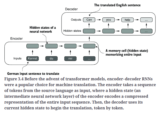
编码器-解码器RNN结构的主要局限性在于:在解码过程中,RNN无法直接访问编码器生成的较早的隐藏状态,只能依赖当前隐藏状态来包含所有相关信息。这可能导致上下文信息的丢失,尤其是在复杂句子中,当依赖关系跨越较长距离时,模型难以保持完整的语义理解。
3.Capturing data dependencies with attention mechanisms
尽管RNN在翻译短句时表现良好,但对于较长文本,其效果较差,因为它无法直接访问输入中的先前单词。
因此,研究人员在2014年提出了Bahdanau注意力机制。该机制对编码器-解码器RNN进行了改进,使解码器在每个解码步骤能够选择性地访问输入序列的不同部分,如Fig3.5所示。
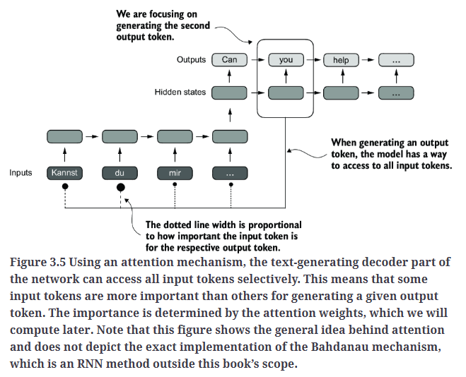
使用注意力机制后,文本生成过程中的解码器可以选择性地访问所有输入token。这意味着,对于生成特定的输出token,某些输入token比其他token更重要。虚线黑点的大小表示该输入token对当前输出token的重要性。注意力权重决定了输入token的重要程度,我们将在后续计算这些权重。Fig3.5展示了注意力机制的基本概念,但并未严格呈现Bahdanau机制的具体实现。
有趣的是,仅仅三年后,研究人员发现,构建用于自然语言处理的深度神经网络并不需要RNN架构。他们提出了原始transformer架构,其中包含了一种受Bahdanau注意力机制启发的自注意力机制。
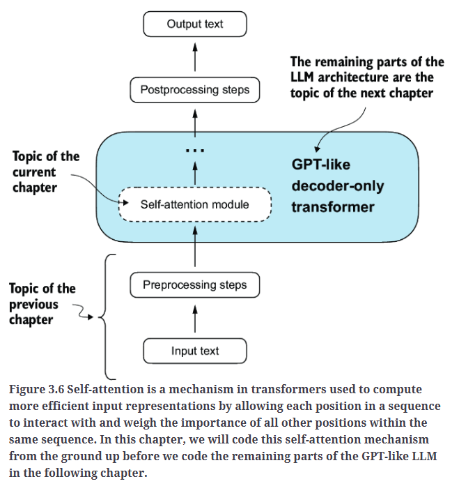
自注意力机制使输入序列中的每个位置在计算序列表示时,能够考虑并关注同一序列中的所有其他位置的相关性。自注意力是基于transformer架构的现代LLM(如GPT系列)的核心组件。
自注意力机制如Fig3.6所示。
4.Attending to different parts of the input with self-attention
4.1.A simple self-attention mechanism without trainable weights
让我们首先实现一个简化版本的自注意力机制,它不包含任何可训练权重,如Fig3.7所示。
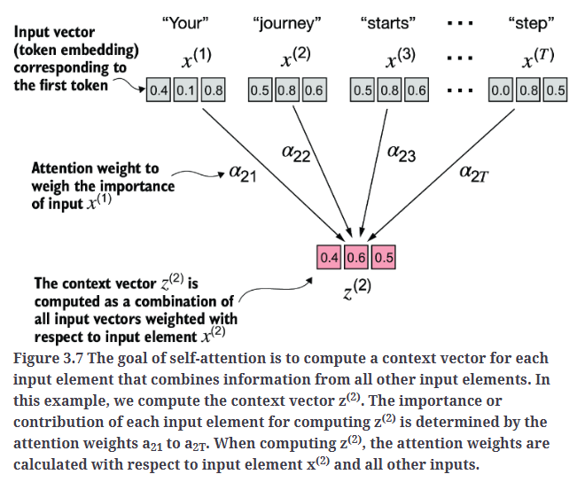
自注意力的目标是计算每个输入元素的上下文向量(context vector),该向量结合了来自所有其他输入元素的信息。在Fig3.7中,$z^{(2)}$是$x^{(2)}$对应的上下文向量。
1
2
3
4
5
6
7
8
9
10
import torch

inputs = torch.tensor(
  [[0.43, 0.15, 0.89], # Your     (x^1)
   [0.55, 0.87, 0.66], # journey  (x^2)
   [0.57, 0.85, 0.64], # starts   (x^3)
   [0.22, 0.58, 0.33], # with     (x^4)
   [0.77, 0.25, 0.10], # one      (x^5)
   [0.05, 0.80, 0.55]] # step     (x^6)
)
实现自注意力的第一步是计算中间值$w$,即注意力分数,如Fig3.8所示。由于空间限制,Fig3.8中的输入张量值都是被截断的。
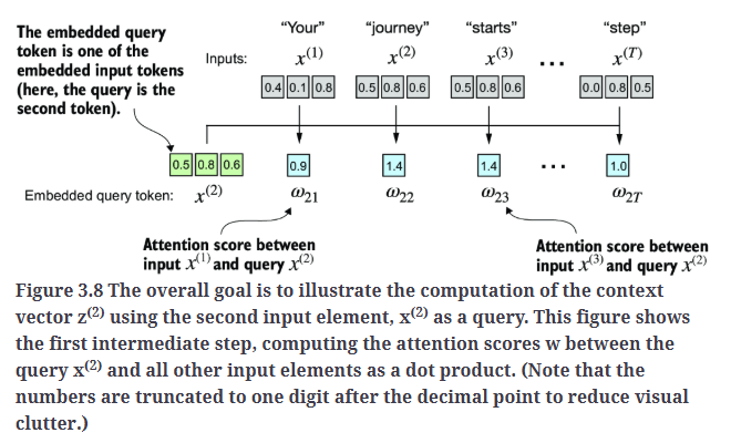
在Fig3.8中,$x^{(2)}$作为query token,计算其与所有输入元素之间的注意力分数$w$。注意力分数是通过点积计算得出的。数值都做了截断处理。比如$w_{21}$的计算为:
\[w_{21} = (0.43 \times 0.55) + (0.15 \times 0.87) + (0.89 \times 0.66) = 0.9544 \approx 0.9\]代码实现:
1
2
3
4
5
6
7
query = inputs[1]  # 2nd input token is the query

attn_scores_2 = torch.empty(inputs.shape[0])
for i, x_i in enumerate(inputs):
    attn_scores_2[i] = torch.dot(x_i, query) # dot product (transpose not necessary here since they are 1-dim vectors)

print(attn_scores_2) #tensor([0.9544, 1.4950, 1.4754, 0.8434, 0.7070, 1.0865])
点积值越高,表示两个元素之间的相似度越高,从而产生更高的注意力分数。
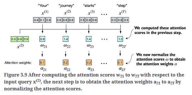
下一步,如Fig3.9所示,对先前计算的注意力分数进行归一化。归一化的主要目标是使所有注意力权重的总和等于1。这种归一化方式是一种惯例,有助于提高注意力权重的可解释性,同时保持LLM训练的稳定性。
1
2
3
4
attn_weights_2_tmp = attn_scores_2 / attn_scores_2.sum()

print("Attention weights:", attn_weights_2_tmp) #Attention weights: tensor([0.1455, 0.2278, 0.2249, 0.1285, 0.1077, 0.1656])
print("Sum:", attn_weights_2_tmp.sum()) #Sum: tensor(1.0000)
在实际应用中,更常见且推荐使用softmax函数进行归一化。这种方法能够更好地处理极端值,并在训练过程中提供更优的梯度特性。代码实现:
1
2
3
4
5
6
7
def softmax_naive(x):
    return torch.exp(x) / torch.exp(x).sum(dim=0)

attn_weights_2_naive = softmax_naive(attn_scores_2)

print("Attention weights:", attn_weights_2_naive) #Attention weights: tensor([0.1385, 0.2379, 0.2333, 0.1240, 0.1082, 0.1581])
print("Sum:", attn_weights_2_naive.sum()) #Sum: tensor(1.)
此外,softmax函数确保注意力权重始终为正值,这使得输出可以被解释为概率或相对重要性。在这种情况下,较高的权重表示更高的重要性。
请注意,这种朴素的softmax实现(softmax_naive)在处理过大或过小的输入值时,可能会遇到数值不稳定的问题,例如上溢(overflow)或下溢(underflow)。因此,在实际应用中,建议使用PyTorch提供的softmax实现,该实现经过广泛优化,在性能和稳定性方面更加可靠:
1
2
3
4
attn_weights_2 = torch.softmax(attn_scores_2, dim=0)

print("Attention weights:", attn_weights_2) #Attention weights: tensor([0.1385, 0.2379, 0.2333, 0.1240, 0.1082, 0.1581])
print("Sum:", attn_weights_2.sum()) #Sum: tensor(1.)
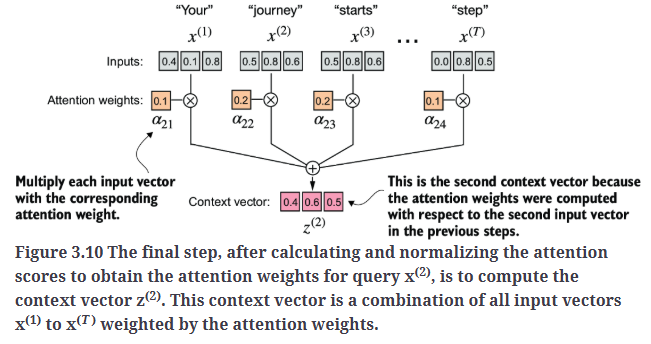
现在,我们已经计算出了归一化的注意力权重,接下来便可以计算上下文向量了,如Fig3.10所示。
1
2
3
4
5
6
7
query = inputs[1] # 2nd input token is the query

context_vec_2 = torch.zeros(query.shape)
for i,x_i in enumerate(inputs):
    context_vec_2 += attn_weights_2[i]*x_i

print(context_vec_2) #tensor([0.4419, 0.6515, 0.5683])
接下来,我们将同时计算所有上下文向量。
4.2.Computing attention weights for all input tokens
到目前为止,我们已经计算了$x^{(2)}$的注意力权重和上下文向量,如Fig3.11中的高亮行所示。现在,让我们扩展这一计算过程,以便计算所有输入的注意力权重和上下文向量。
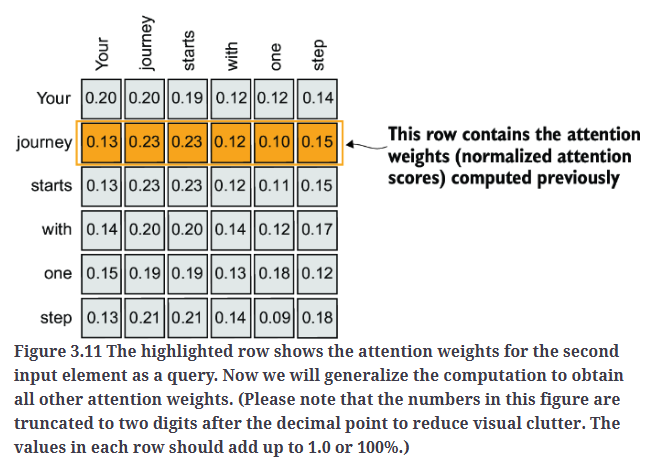
Fig3.11中,每一行代表一个输入元素作为query时的注意力权重分布。所有数值均被截断至小数点后两位。每一行的总和应等于1.0。
我们仍然遵循之前的三个步骤(见Fig3.12),但在代码中做了一些修改,以同时计算所有上下文向量。
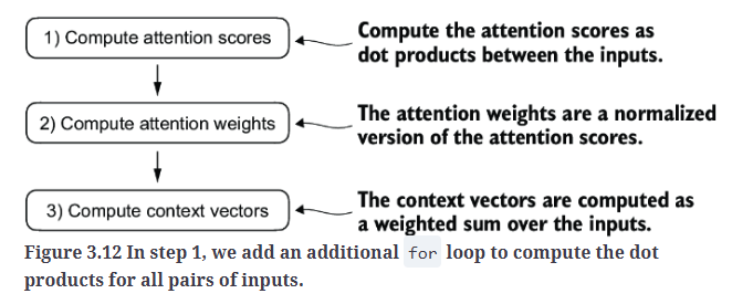
第一步:计算点积得到注意力分数。
1
2
3
4
5
6
7
8
9
10
11
12
#较慢的实现方式,for循环:
attn_scores = torch.empty(6, 6)

for i, x_i in enumerate(inputs):
    for j, x_j in enumerate(inputs):
        attn_scores[i, j] = torch.dot(x_i, x_j)

print(attn_scores)

#较快的实现方式,矩阵乘法:
attn_scores = inputs @ inputs.T
print(attn_scores)
输出为:
1
2
3
4
5
6
tensor([[0.9995, 0.9544, 0.9422, 0.4753, 0.4576, 0.6310],
        [0.9544, 1.4950, 1.4754, 0.8434, 0.7070, 1.0865],
        [0.9422, 1.4754, 1.4570, 0.8296, 0.7154, 1.0605],
        [0.4753, 0.8434, 0.8296, 0.4937, 0.3474, 0.6565],
        [0.4576, 0.7070, 0.7154, 0.3474, 0.6654, 0.2935],
        [0.6310, 1.0865, 1.0605, 0.6565, 0.2935, 0.9450]])
第二步:归一化注意力分数得到注意力权重。
1
2
attn_weights = torch.softmax(attn_scores, dim=-1)
print(attn_weights)
输出为:
1
2
3
4
5
6
tensor([[0.2098, 0.2006, 0.1981, 0.1242, 0.1220, 0.1452],
        [0.1385, 0.2379, 0.2333, 0.1240, 0.1082, 0.1581],
        [0.1390, 0.2369, 0.2326, 0.1242, 0.1108, 0.1565],
        [0.1435, 0.2074, 0.2046, 0.1462, 0.1263, 0.1720],
        [0.1526, 0.1958, 0.1975, 0.1367, 0.1879, 0.1295],
        [0.1385, 0.2184, 0.2128, 0.1420, 0.0988, 0.1896]])
第三步:计算所有的上下文向量。
1
2
all_context_vecs = attn_weights @ inputs
print(all_context_vecs)
输出为:
1
2
3
4
5
6
tensor([[0.4421, 0.5931, 0.5790],
        [0.4419, 0.6515, 0.5683],
        [0.4431, 0.6496, 0.5671],
        [0.4304, 0.6298, 0.5510],
        [0.4671, 0.5910, 0.5266],
        [0.4177, 0.6503, 0.5645]])
至此,我们完成了简单自注意力机制。接下来,我们将引入可训练权重,使LLM能够从数据中学习,并在特定任务上提升性能。
5.Implementing self-attention with trainable weights
我们的下一步是实现原始transformer结构、GPT模型以及大多数主流LLM中使用的自注意力机制。该自注意力机制也被称为缩放点积注意力(scaled dot-product attention)。
与我们之前实现的基础自注意力机制相比,最显著的区别是引入了权重矩阵,这些矩阵会在模型训练过程中进行更新。这些可训练的权重矩阵至关重要,因为它们使模型(特别是模型内部的注意力模块)能够学习如何生成“优质”的上下文向量。
5.1.Computing the attention weights step by step
首先引入三个可训练的权重矩阵:$W_q$、$W_k$和$W_v$。这三个权重矩阵可以将输入$x^{(i)}$分别映射为query向量、key向量和value向量,如Fig3.14所示。
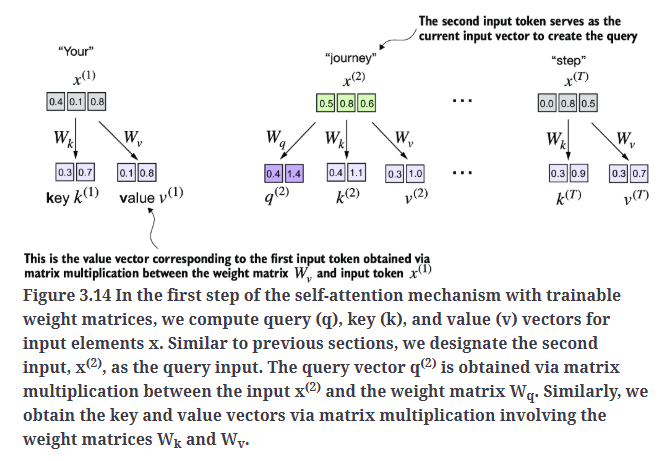
同样的,我们首先仅计算一个上下文向量$z^{(2)}$作为示例。随后,我们将修改代码,以计算所有上下文向量。
1
2
3
4
5
6
7
8
9
x_2 = inputs[1] # second input element
d_in = inputs.shape[1] # the input embedding size, d=3
d_out = 2 # the output embedding size, d=2

#随机初始化3个权重矩阵
torch.manual_seed(123)
W_query = torch.nn.Parameter(torch.rand(d_in, d_out), requires_grad=False)
W_key   = torch.nn.Parameter(torch.rand(d_in, d_out), requires_grad=False)
W_value = torch.nn.Parameter(torch.rand(d_in, d_out), requires_grad=False)
我们将requires_grad=False设置为不计算梯度,以减少输出中的冗余信息。但如果我们要在模型训练过程中更新这些权重矩阵,则应将requires_grad=True,使其在训练时可被优化。
1
2
3
4
5
6
7
8
9
10
11
query_2 = x_2 @ W_query # _2 because it's with respect to the 2nd input element
key_2 = x_2 @ W_key
value_2 = x_2 @ W_value

print(query_2) #tensor([0.4306, 1.4551])

keys = inputs @ W_key
values = inputs @ W_value

print("keys.shape:", keys.shape) #keys.shape: torch.Size([6, 2])
print("values.shape:", values.shape) #values.shape: torch.Size([6, 2])
1
2
attn_scores_2 = query_2 @ keys.T # All attention scores for given query
print(attn_scores_2) #tensor([1.2705, 1.8524, 1.8111, 1.0795, 0.5577, 1.5440])
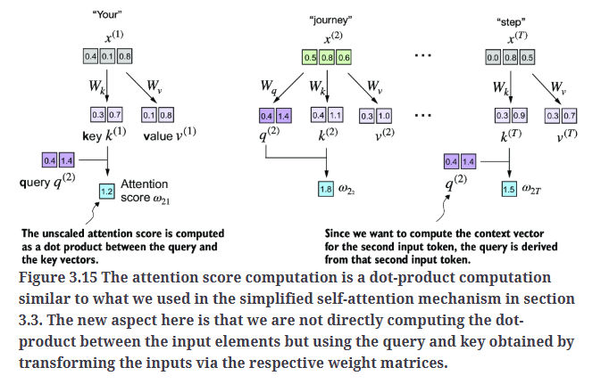
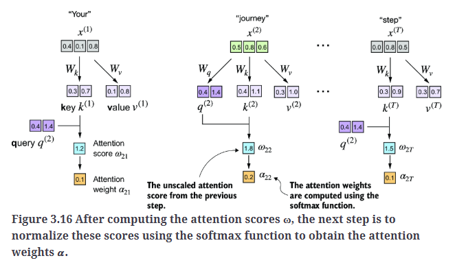
对注意力分数进行缩放并使用softmax函数归一化得到注意力权重,如Fig3.16所示。
1
2
3
d_k = keys.shape[1]
attn_weights_2 = torch.softmax(attn_scores_2 / d_k**0.5, dim=-1)
print(attn_weights_2) #tensor([0.1500, 0.2264, 0.2199, 0.1311, 0.0906, 0.1820])
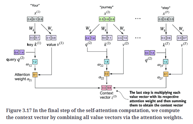
1
2
context_vec_2 = attn_weights_2 @ values
print(context_vec_2) #tensor([0.3061, 0.8210])
至此,我们计算得到了上下文向量$z^{(2)}$。然后,我们将修改代码来一次性计算所有的上下文向量。
5.2.Implementing a compact self-attention Python class
将上述那些代码封装到一个Python类中:
1
2
3
4
5
6
7
8
9
10
11
12
13
14
15
16
17
18
19
20
21
22
23
24
25
26
import torch.nn as nn

class SelfAttention_v1(nn.Module):

    def __init__(self, d_in, d_out):
        super().__init__()
        self.W_query = nn.Parameter(torch.rand(d_in, d_out))
        self.W_key   = nn.Parameter(torch.rand(d_in, d_out))
        self.W_value = nn.Parameter(torch.rand(d_in, d_out))

    def forward(self, x):
        keys = x @ self.W_key
        queries = x @ self.W_query
        values = x @ self.W_value

        attn_scores = queries @ keys.T # omega
        attn_weights = torch.softmax(
            attn_scores / keys.shape[-1]**0.5, dim=-1
        )

        context_vec = attn_weights @ values
        return context_vec

torch.manual_seed(123)
sa_v1 = SelfAttention_v1(d_in, d_out)
print(sa_v1(inputs))
输出为:
1
2
3
4
5
6
tensor([[0.2996, 0.8053],
        [0.3061, 0.8210],
        [0.3058, 0.8203],
        [0.2948, 0.7939],
        [0.2927, 0.7891],
        [0.2990, 0.8040]], grad_fn=<MmBackward0>)
在这段PyTorch代码中,SelfAttention_v1是一个继承自nn.Module的类。nn.Module是PyTorch模型的基本构建模块,它提供了创建和管理模型层所需的功能。
Fig3.18总结了我们刚实现的自注意力机制:
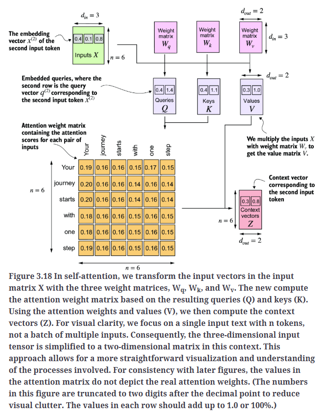
我们可以使用PyTorch的nn.Linear层进一步优化SelfAttention_v1的实现。当禁用偏置单元(bias units)时,nn.Linear本质上执行的是矩阵乘法。此外,相较于手动使用nn.Parameter(torch.rand(...))进行权重初始化,nn.Linear具有优化的权重初始化方案,这有助于提高模型训练的稳定性和效果。
1
2
3
4
5
6
7
8
9
10
11
12
13
14
15
16
17
18
19
20
21
22
class SelfAttention_v2(nn.Module):

    def __init__(self, d_in, d_out, qkv_bias=False):
        super().__init__()
        self.W_query = nn.Linear(d_in, d_out, bias=qkv_bias)
        self.W_key   = nn.Linear(d_in, d_out, bias=qkv_bias)
        self.W_value = nn.Linear(d_in, d_out, bias=qkv_bias)

    def forward(self, x):
        keys = self.W_key(x)
        queries = self.W_query(x)
        values = self.W_value(x)

        attn_scores = queries @ keys.T
        attn_weights = torch.softmax(attn_scores / keys.shape[-1]**0.5, dim=-1)

        context_vec = attn_weights @ values
        return context_vec

torch.manual_seed(789)
sa_v2 = SelfAttention_v2(d_in, d_out)
print(sa_v2(inputs))
输出为:
1
2
3
4
5
6
tensor([[-0.0739,  0.0713],
        [-0.0748,  0.0703],
        [-0.0749,  0.0702],
        [-0.0760,  0.0685],
        [-0.0763,  0.0679],
        [-0.0754,  0.0693]], grad_fn=<MmBackward0>)
请注意,SelfAttention_v1和SelfAttention_v2的输出不同,因为它们的权重矩阵使用了不同的初始化方式,nn.Linear采用了更复杂的权重初始化方案。
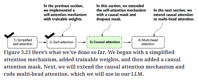
接下来,我们将对自注意力机制进行增强,重点加入因果性(causal)和多头(multi-head)元素。因果性的引入涉及修改注意力机制,以防止模型访问序列中的未来信息,这对于语言建模等任务至关重要,因为每个单词的预测应仅依赖于前面的单词。
6.Hiding future words with causal attention
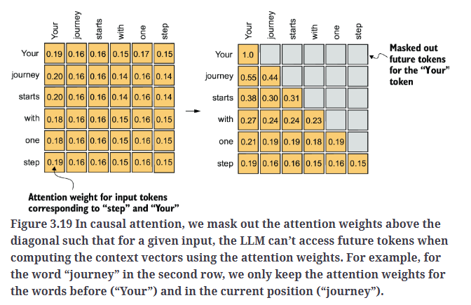
在许多LLM任务中,自注意力机制在预测序列中的下一个token时,通常只能考虑当前位置之前出现的token。因果注意力(causal attention),也称为掩码注意力(masked attention),是一种特殊的自注意力形式。它限制模型在计算注意力分数时,仅能考虑序列中的先前和当前输入,而标准自注意力机制则允许访问整个输入序列。
如Fig3.19所示,我们屏蔽对角线以上的注意力权重,并对未屏蔽的注意力权重进行归一化,使得每一行的注意力权重总和为1。
6.1.Applying a causal attention mask
为了应用因果注意力掩码并获得屏蔽后的注意力权重,我们将按照Fig3.20总结的步骤进行实现。
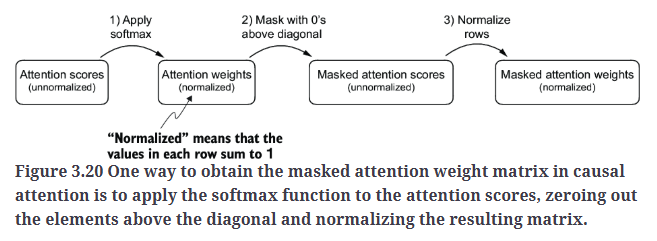
第一步,和之前一样,计算注意力权重。
1
2
3
4
5
6
7
8
# Reuse the query and key weight matrices of the
# SelfAttention_v2 object from the previous section for convenience
queries = sa_v2.W_query(inputs)
keys = sa_v2.W_key(inputs)
attn_scores = queries @ keys.T

attn_weights = torch.softmax(attn_scores / keys.shape[-1]**0.5, dim=-1)
print(attn_weights)
输出为:
1
2
3
4
5
6
7
tensor([[0.1921, 0.1646, 0.1652, 0.1550, 0.1721, 0.1510],
        [0.2041, 0.1659, 0.1662, 0.1496, 0.1665, 0.1477],
        [0.2036, 0.1659, 0.1662, 0.1498, 0.1664, 0.1480],
        [0.1869, 0.1667, 0.1668, 0.1571, 0.1661, 0.1564],
        [0.1830, 0.1669, 0.1670, 0.1588, 0.1658, 0.1585],
        [0.1935, 0.1663, 0.1666, 0.1542, 0.1666, 0.1529]],
       grad_fn=<SoftmaxBackward0>)
第二步,创建掩码,使对角线以上的值为零。
1
2
3
context_length = attn_scores.shape[0]
mask_simple = torch.tril(torch.ones(context_length, context_length))
print(mask_simple)
输出为:
1
2
3
4
5
6
tensor([[1., 0., 0., 0., 0., 0.],
        [1., 1., 0., 0., 0., 0.],
        [1., 1., 1., 0., 0., 0.],
        [1., 1., 1., 1., 0., 0.],
        [1., 1., 1., 1., 1., 0.],
        [1., 1., 1., 1., 1., 1.]])
应用掩码:
1
2
masked_simple = attn_weights*mask_simple
print(masked_simple)
输出为:
1
2
3
4
5
6
7
tensor([[0.1921, 0.0000, 0.0000, 0.0000, 0.0000, 0.0000],
        [0.2041, 0.1659, 0.0000, 0.0000, 0.0000, 0.0000],
        [0.2036, 0.1659, 0.1662, 0.0000, 0.0000, 0.0000],
        [0.1869, 0.1667, 0.1668, 0.1571, 0.0000, 0.0000],
        [0.1830, 0.1669, 0.1670, 0.1588, 0.1658, 0.0000],
        [0.1935, 0.1663, 0.1666, 0.1542, 0.1666, 0.1529]],
       grad_fn=<MulBackward0>)
第三步,重新归一化。
1
2
3
row_sums = masked_simple.sum(dim=-1, keepdim=True)
masked_simple_norm = masked_simple / row_sums
print(masked_simple_norm)
输出为:
1
2
3
4
5
6
7
tensor([[1.0000, 0.0000, 0.0000, 0.0000, 0.0000, 0.0000],
        [0.5517, 0.4483, 0.0000, 0.0000, 0.0000, 0.0000],
        [0.3800, 0.3097, 0.3103, 0.0000, 0.0000, 0.0000],
        [0.2758, 0.2460, 0.2462, 0.2319, 0.0000, 0.0000],
        [0.2175, 0.1983, 0.1984, 0.1888, 0.1971, 0.0000],
        [0.1935, 0.1663, 0.1666, 0.1542, 0.1666, 0.1529]],
       grad_fn=<DivBackward0>)
Fig3.21给出了一种步骤更少、更高效的实现方式。
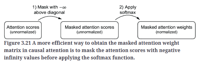
softmax函数会将$-\infty$视为0,因为从数学上讲,$e^{-\infty}$趋近于0。
1
2
3
mask = torch.triu(torch.ones(context_length, context_length), diagonal=1)
masked = attn_scores.masked_fill(mask.bool(), -torch.inf)
print(masked)
输出为:
1
2
3
4
5
6
7
tensor([[0.2899,   -inf,   -inf,   -inf,   -inf,   -inf],
        [0.4656, 0.1723,   -inf,   -inf,   -inf,   -inf],
        [0.4594, 0.1703, 0.1731,   -inf,   -inf,   -inf],
        [0.2642, 0.1024, 0.1036, 0.0186,   -inf,   -inf],
        [0.2183, 0.0874, 0.0882, 0.0177, 0.0786,   -inf],
        [0.3408, 0.1270, 0.1290, 0.0198, 0.1290, 0.0078]],
       grad_fn=<MaskedFillBackward0>)
1
2
attn_weights = torch.softmax(masked / keys.shape[-1]**0.5, dim=-1)
print(attn_weights)
输出为:
1
2
3
4
5
6
7
tensor([[1.0000, 0.0000, 0.0000, 0.0000, 0.0000, 0.0000],
        [0.5517, 0.4483, 0.0000, 0.0000, 0.0000, 0.0000],
        [0.3800, 0.3097, 0.3103, 0.0000, 0.0000, 0.0000],
        [0.2758, 0.2460, 0.2462, 0.2319, 0.0000, 0.0000],
        [0.2175, 0.1983, 0.1984, 0.1888, 0.1971, 0.0000],
        [0.1935, 0.1663, 0.1666, 0.1542, 0.1666, 0.1529]],
       grad_fn=<SoftmaxBackward0>)
接下来,我们将介绍因果注意力机制的另一个小优化,它在训练LLM时有助于减少过拟合。
6.2.Masking additional attention weights with dropout
在训练过程中使用dropout防止过拟合,在推理阶段dropout被禁用。
在transformer框架中,包括GPT等模型,注意力机制中的dropout通常应用在两个特定阶段:1)计算注意力权重之后;2)将注意力权重应用到value向量之后。我们将采用第一种方式,如Fig3.22所示,因为这是实践中更常见的做法。
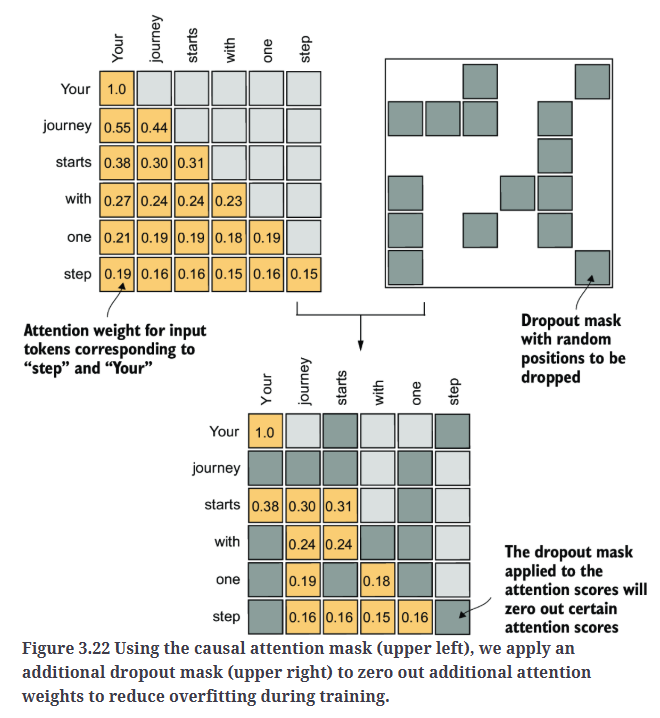
在接下来的代码示例中,我们使用50%的dropout率,这意味着会屏蔽掉一半的注意力权重。
1
2
3
4
5
torch.manual_seed(123)
dropout = torch.nn.Dropout(0.5) # dropout rate of 50%
example = torch.ones(6, 6) # create a matrix of ones

print(dropout(example))
输出为:
1
2
3
4
5
6
tensor([[2., 2., 0., 2., 2., 0.],
        [0., 0., 0., 2., 0., 2.],
        [2., 2., 2., 2., 0., 2.],
        [0., 2., 2., 0., 0., 2.],
        [0., 2., 0., 2., 0., 2.],
        [0., 2., 2., 2., 2., 0.]])
当对注意力权重矩阵应用50%的dropout率时,矩阵中一半的元素会被随机设置为零。为了补偿有效元素的减少,矩阵中剩余元素的值会被放大,缩放因子为1 / (1 - dropout_rate),本例中为1/0.5=2。这种缩放对于保持注意力权重的整体平衡至关重要,确保注意力机制的平均影响力在训练和推理阶段保持一致。
1
2
torch.manual_seed(123)
print(dropout(attn_weights))
输出为:
1
2
3
4
5
6
7
tensor([[2.0000, 0.0000, 0 .0000, 0.0000, 0.0000, 0.0000],
        [0.0000, 0.0000, 0.0000, 0.0000, 0.0000, 0.0000],
        [0.7599, 0.6194, 0.6206, 0.0000, 0.0000, 0.0000],
        [0.0000, 0.4921, 0.4925, 0.0000, 0.0000, 0.0000],
        [0.0000, 0.3966, 0.0000, 0.3775, 0.0000, 0.0000],
        [0.0000, 0.3327, 0.3331, 0.3084, 0.3331, 0.0000]],
       grad_fn=<MulBackward0>)
请注意,dropout的输出结果可能会因操作系统不同而有所差异,参见:https://github.com/pytorch/pytorch/issues/121595。
6.3.Implementing a compact causal attention class
现在我们将因果注意力和dropout机制整合到第5部分的Python类中。此外,我们还需要确保代码能够处理多个输入的batch。
为了简化,我们将一个输入复制为两份,作为一个batch:
1
2
3
batch = torch.stack((inputs, inputs), dim=0)
# 2 inputs with 6 tokens each, and each token has embedding dimension 3
print(batch.shape) #torch.Size([2, 6, 3])
下面的CausalAttention类与我们之前实现的SelfAttention类类似,不同之处在于新增了dropout机制和因果掩码。
1
2
3
4
5
6
7
8
9
10
11
12
13
14
15
16
17
18
19
20
21
22
23
24
25
26
27
28
29
30
31
32
33
34
35
36
37
38
class CausalAttention(nn.Module):

    def __init__(self, d_in, d_out, context_length,
                 dropout, qkv_bias=False):
        super().__init__()
        self.d_out = d_out
        self.W_query = nn.Linear(d_in, d_out, bias=qkv_bias)
        self.W_key   = nn.Linear(d_in, d_out, bias=qkv_bias)
        self.W_value = nn.Linear(d_in, d_out, bias=qkv_bias)
        self.dropout = nn.Dropout(dropout) # New
        self.register_buffer('mask', torch.triu(torch.ones(context_length, context_length), diagonal=1)) # New

    def forward(self, x):
        b, num_tokens, d_in = x.shape # New batch dimension b
        keys = self.W_key(x)
        queries = self.W_query(x)
        values = self.W_value(x)

        attn_scores = queries @ keys.transpose(1, 2) # Changed transpose
        attn_scores.masked_fill_(  # New, _ ops are in-place
            self.mask.bool()[:num_tokens, :num_tokens], -torch.inf)  # `:num_tokens` to account for cases where the number of tokens in the batch is smaller than the supported context_size
        attn_weights = torch.softmax(
            attn_scores / keys.shape[-1]**0.5, dim=-1
        )
        attn_weights = self.dropout(attn_weights) # New

        context_vec = attn_weights @ values
        return context_vec

torch.manual_seed(123)

context_length = batch.shape[1]
ca = CausalAttention(d_in, d_out, context_length, 0.0)

context_vecs = ca(batch)

print(context_vecs)
print("context_vecs.shape:", context_vecs.shape)
输出为:
1
2
3
4
5
6
7
8
9
10
11
12
13
14
tensor([[[-0.4519,  0.2216],
         [-0.5874,  0.0058],
         [-0.6300, -0.0632],
         [-0.5675, -0.0843],
         [-0.5526, -0.0981],
         [-0.5299, -0.1081]],

        [[-0.4519,  0.2216],
         [-0.5874,  0.0058],
         [-0.6300, -0.0632],
         [-0.5675, -0.0843],
         [-0.5526, -0.0981],
         [-0.5299, -0.1081]]], grad_fn=<UnsafeViewBackward0>)
context_vecs.shape: torch.Size([2, 6, 2])
在PyTorch中,register_buffer并不是所有情况下都必须使用,但在这里具有几个重要的优势。例如,当我们在LLM中使用CausalAttention类时,所有缓冲区(buffers)都会自动随模型移动到合适的设备(CPU或GPU),这在训练LLM时尤为重要。这样,我们无需手动确保这些张量与模型参数位于同一设备上,从而避免设备不匹配错误。
7.Extending single-head attention to multi-head attention
单个因果注意力模块可以被视为单头注意力。
7.1.Stacking multiple single-head attention layers
尽管使用多个自注意力机制会增加计算量,但这对于复杂模式识别至关重要,也是基于transformer的LLM能够高效学习复杂结构的关键。
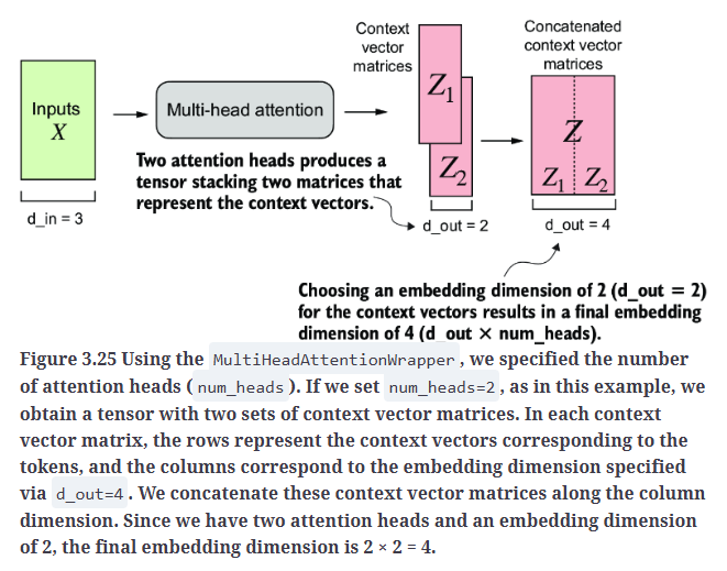
Fig3.24展示了多头注意力模块的结构,它由多个单头注意力模块组成。
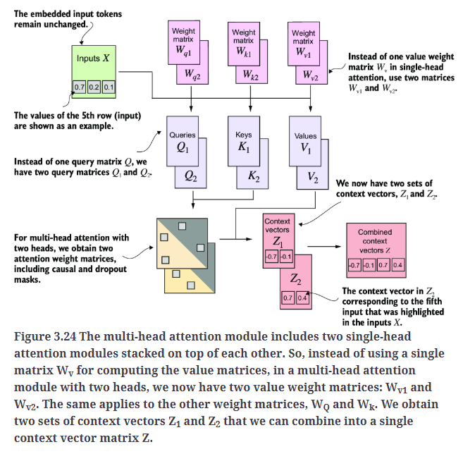
在代码实现上,我们可以创建一个简单的MultiHeadAttentionWrapper类,它通过堆叠多个CausalAttention模块来实现多头注意力机制。
1
2
3
4
5
6
7
8
9
10
11
12
13
14
15
16
17
18
19
20
21
22
23
24
25
class MultiHeadAttentionWrapper(nn.Module):

    def __init__(self, d_in, d_out, context_length, dropout, num_heads, qkv_bias=False):
        super().__init__()
        self.heads = nn.ModuleList(
            [CausalAttention(d_in, d_out, context_length, dropout, qkv_bias)
             for _ in range(num_heads)]
        )

    def forward(self, x):
        return torch.cat([head(x) for head in self.heads], dim=-1)


torch.manual_seed(123)

context_length = batch.shape[1] # This is the number of tokens
d_in, d_out = 3, 2
mha = MultiHeadAttentionWrapper(
    d_in, d_out, context_length, 0.0, num_heads=2
)

context_vecs = mha(batch)

print(context_vecs)
print("context_vecs.shape:", context_vecs.shape)
输出为:
1
2
3
4
5
6
7
8
9
10
11
12
13
14
tensor([[[-0.4519,  0.2216,  0.4772,  0.1063],
         [-0.5874,  0.0058,  0.5891,  0.3257],
         [-0.6300, -0.0632,  0.6202,  0.3860],
         [-0.5675, -0.0843,  0.5478,  0.3589],
         [-0.5526, -0.0981,  0.5321,  0.3428],
         [-0.5299, -0.1081,  0.5077,  0.3493]],

        [[-0.4519,  0.2216,  0.4772,  0.1063],
         [-0.5874,  0.0058,  0.5891,  0.3257],
         [-0.6300, -0.0632,  0.6202,  0.3860],
         [-0.5675, -0.0843,  0.5478,  0.3589],
         [-0.5526, -0.0981,  0.5321,  0.3428],
         [-0.5299, -0.1081,  0.5077,  0.3493]]], grad_fn=<CatBackward0>)
context_vecs.shape: torch.Size([2, 6, 4])
7.2.Implementing multi-head attention with weight splits
本部分我们将MultiHeadAttentionWrapper类和CausalAttention类合并成一个统一的MultiHeadAttention类,此外,我们还将进行一些优化,以更高效地实现多头注意力。
1
2
3
4
5
6
7
8
9
10
11
12
13
14
15
16
17
18
19
20
21
22
23
24
25
26
27
28
29
30
31
32
33
34
35
36
37
38
39
40
41
42
43
44
45
46
47
48
49
50
51
52
53
54
55
56
57
58
59
60
61
62
63
64
65
66
67
68
69
70
class MultiHeadAttention(nn.Module):
    def __init__(self, d_in, d_out, context_length, dropout, num_heads, qkv_bias=False):
        super().__init__()
        assert (d_out % num_heads == 0), \
            "d_out must be divisible by num_heads"

        self.d_out = d_out
        self.num_heads = num_heads
        self.head_dim = d_out // num_heads # Reduce the projection dim to match desired output dim

        self.W_query = nn.Linear(d_in, d_out, bias=qkv_bias)
        self.W_key = nn.Linear(d_in, d_out, bias=qkv_bias)
        self.W_value = nn.Linear(d_in, d_out, bias=qkv_bias)
        self.out_proj = nn.Linear(d_out, d_out)  # Linear layer to combine head outputs
        self.dropout = nn.Dropout(dropout)
        self.register_buffer(
            "mask",
            torch.triu(torch.ones(context_length, context_length),
                       diagonal=1)
        )

    def forward(self, x):
        b, num_tokens, d_in = x.shape

        keys = self.W_key(x) # Shape: (b, num_tokens, d_out)
        queries = self.W_query(x)
        values = self.W_value(x)

        # We implicitly split the matrix by adding a `num_heads` dimension
        # Unroll last dim: (b, num_tokens, d_out) -> (b, num_tokens, num_heads, head_dim)
        keys = keys.view(b, num_tokens, self.num_heads, self.head_dim)
        values = values.view(b, num_tokens, self.num_heads, self.head_dim)
        queries = queries.view(b, num_tokens, self.num_heads, self.head_dim)

        # Transpose: (b, num_tokens, num_heads, head_dim) -> (b, num_heads, num_tokens, head_dim)
        keys = keys.transpose(1, 2)
        queries = queries.transpose(1, 2)
        values = values.transpose(1, 2)

        # Compute scaled dot-product attention (aka self-attention) with a causal mask
        attn_scores = queries @ keys.transpose(2, 3)  # Dot product for each head

        # Original mask truncated to the number of tokens and converted to boolean
        mask_bool = self.mask.bool()[:num_tokens, :num_tokens]

        # Use the mask to fill attention scores
        attn_scores.masked_fill_(mask_bool, -torch.inf)

        attn_weights = torch.softmax(attn_scores / keys.shape[-1]**0.5, dim=-1)
        attn_weights = self.dropout(attn_weights)

        # Shape: (b, num_tokens, num_heads, head_dim)
        context_vec = (attn_weights @ values).transpose(1, 2)

        # Combine heads, where self.d_out = self.num_heads * self.head_dim
        context_vec = context_vec.contiguous().view(b, num_tokens, self.d_out)
        context_vec = self.out_proj(context_vec) # optional projection

        return context_vec

torch.manual_seed(123)

batch_size, context_length, d_in = batch.shape
d_out = 2
mha = MultiHeadAttention(d_in, d_out, context_length, 0.0, num_heads=2)

context_vecs = mha(batch)

print(context_vecs)
print("context_vecs.shape:", context_vecs.shape)
输出为:
1
2
3
4
5
6
7
8
9
10
11
12
13
14
tensor([[[0.3190, 0.4858],
         [0.2943, 0.3897],
         [0.2856, 0.3593],
         [0.2693, 0.3873],
         [0.2639, 0.3928],
         [0.2575, 0.4028]],

        [[0.3190, 0.4858],
         [0.2943, 0.3897],
         [0.2856, 0.3593],
         [0.2693, 0.3873],
         [0.2639, 0.3928],
         [0.2575, 0.4028]]], grad_fn=<ViewBackward0>)
context_vecs.shape: torch.Size([2, 6, 2])
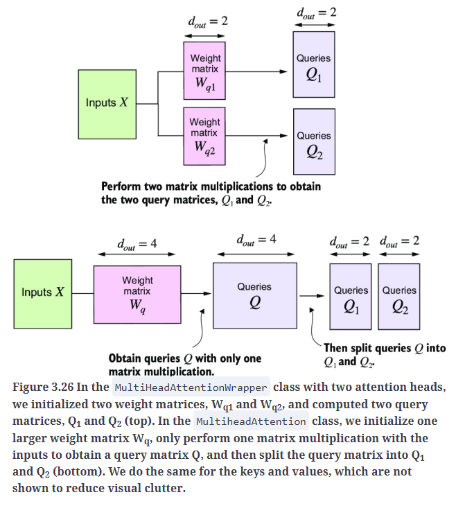
Fig3.26上是MultiHeadAttentionWrapper类的实现思路,Fig3.26下是MultiheadAttention类的实现思路。