【从零开始构建大语言模型】系列博客为”Build a Large Language Model (From Scratch)”一书的个人读书笔记。
- 原书链接:Build a Large Language Model (From Scratch)。
- 官方示例代码:LLMs-from-scratch。
本文为原创文章,未经本人允许,禁止转载。转载请注明出处。
1.Implementing a GPT model from scratch to generate text

2.Coding an LLM architecture
Fig4.2展示了一个类似GPT的LLM的整体视图,并突出显示了其主要组成部分。

之前,我们使用了较小的嵌入维度,以保持简洁。现在,我们将扩展到一个小型GPT-2模型的规模,具体来说,是最小版本,包含1.24亿个参数。需要注意的是,尽管原始报告提到该模型包含1.17亿个参数,但这一数据后来被更正。
在深度学习和GPT等LLM的背景下,“参数”指的是模型的可训练权重。这些权重本质上是模型的内部变量,在训练过程中通过调整和优化来最小化特定的损失函数。通过这种优化,模型能够从训练数据中学习。
我们通过以下Python字典指定小型GPT-2模型的配置:
1
2
3
4
5
6
7
8
9
GPT_CONFIG_124M = {
    "vocab_size": 50257,    # Vocabulary size
    "context_length": 1024, # Context length
    "emb_dim": 768,         # Embedding dimension
    "n_heads": 12,          # Number of attention heads
    "n_layers": 12,         # Number of layers
    "drop_rate": 0.1,       # Dropout rate
    "qkv_bias": False       # Query-Key-Value bias
}
使用此配置,我们将实现一个如Fig4.3所示的DummyGPTModel(注:是一个空的框架,后续会陆续补全)。这将帮助我们从整体上理解各个部分如何协同工作,并明确需要编写哪些其他组件,以组装完整的GPT模型架构。

1
2
3
4
5
6
7
8
9
10
11
12
13
14
15
16
17
18
19
20
21
22
23
24
25
26
27
28
29
30
31
32
33
34
35
36
37
38
39
40
41
42
43
44
45
46
47
48
49
50
51
import torch
import torch.nn as nn


class DummyGPTModel(nn.Module):
    def __init__(self, cfg):
        super().__init__()
        self.tok_emb = nn.Embedding(cfg["vocab_size"], cfg["emb_dim"])
        self.pos_emb = nn.Embedding(cfg["context_length"], cfg["emb_dim"])
        self.drop_emb = nn.Dropout(cfg["drop_rate"])

        # Use a placeholder for TransformerBlock
        self.trf_blocks = nn.Sequential(
            *[DummyTransformerBlock(cfg) for _ in range(cfg["n_layers"])])

        # Use a placeholder for LayerNorm
        self.final_norm = DummyLayerNorm(cfg["emb_dim"])
        self.out_head = nn.Linear(
            cfg["emb_dim"], cfg["vocab_size"], bias=False
        )

    def forward(self, in_idx):
        batch_size, seq_len = in_idx.shape
        tok_embeds = self.tok_emb(in_idx)
        pos_embeds = self.pos_emb(torch.arange(seq_len, device=in_idx.device))
        x = tok_embeds + pos_embeds
        x = self.drop_emb(x) #注意:这里对输入序列也做了dropout
        x = self.trf_blocks(x) #堆叠多个transformer block
        x = self.final_norm(x) #最终的层归一化
        logits = self.out_head(x) #线性输出层,输出每个单词的概率
        return logits


class DummyTransformerBlock(nn.Module):
    def __init__(self, cfg):
        super().__init__()
        # A simple placeholder

    def forward(self, x):
        # This block does nothing and just returns its input.
        return x


class DummyLayerNorm(nn.Module):
    def __init__(self, normalized_shape, eps=1e-5):
        super().__init__()
        # The parameters here are just to mimic the LayerNorm interface.

    def forward(self, x):
        # This layer does nothing and just returns its input.
        return x
现在让我们从宏观的角度来看数据在GPT模型中的输入和输出流程,如Fig4.4所示。

为了实现这些步骤,我们使用第2章中的tiktoken分词器,对batch(包含两个文本输入)进行分词,以供GPT模型使用:
1
2
3
4
5
6
7
8
9
10
11
12
13
import tiktoken

tokenizer = tiktoken.get_encoding("gpt2")

batch = []

txt1 = "Every effort moves you"
txt2 = "Every day holds a"

batch.append(torch.tensor(tokenizer.encode(txt1)))
batch.append(torch.tensor(tokenizer.encode(txt2)))
batch = torch.stack(batch, dim=0)
print(batch)
输出为:
1
2
tensor([[6109, 3626, 6100,  345],
        [6109, 1110, 6622,  257]])
接下来,我们初始化一个具有1.24亿参数的DummyGPTModel实例,并将分词后的batch喂入模型中:
1
2
3
4
5
6
torch.manual_seed(123)
model = DummyGPTModel(GPT_CONFIG_124M)

logits = model(batch)
print("Output shape:", logits.shape)
print(logits)
输出为:
1
2
3
4
5
6
7
8
9
10
11
Output shape: torch.Size([2, 4, 50257])
tensor([[[-0.9289,  0.2748, -0.7557,  ..., -1.6070,  0.2702, -0.5888],
         [-0.4476,  0.1726,  0.5354,  ..., -0.3932,  1.5285,  0.8557],
         [ 0.5680,  1.6053, -0.2155,  ...,  1.1624,  0.1380,  0.7425],
         [ 0.0447,  2.4787, -0.8843,  ...,  1.3219, -0.0864, -0.5856]],

        [[-1.5474, -0.0542, -1.0571,  ..., -1.8061, -0.4494, -0.6747],
         [-0.8422,  0.8243, -0.1098,  ..., -0.1434,  0.2079,  1.2046],
         [ 0.1355,  1.1858, -0.1453,  ...,  0.0869, -0.1590,  0.1552],
         [ 0.1666, -0.8138,  0.2307,  ...,  2.5035, -0.3055, -0.3083]]],
       grad_fn=<UnsafeViewBackward0>)
3.Normalizing activations with layer normalization
训练具有许多层的深度神经网络有时会面临挑战,比如梯度消失或梯度爆炸等问题。这些问题会导致训练过程不稳定,使得网络难以有效调整其权重,也就是说学习过程很难找到一组能够最小化损失函数的参数(权重)。换句话说,网络难以充分学习数据中的潜在模式,从而无法做出准确的预测或决策。
接下来,我们将实现层归一化来提高神经网络训练的稳定性和效率。层归一化的核心思想是将神经网络某一层的激活值(输出)调整为均值为0、方差为1(也称为单位方差)。这种调整能够加快网络参数收敛到有效的权重范围,并确保训练过程更加稳定可靠。在GPT-2以及现代transformer架构中,通常会在多头注意力模块的前后应用层归一化。层归一化的具体工作方式见Fig4.5。

Fig4.5的实现代码如下:
1
2
3
4
5
6
7
8
torch.manual_seed(123)

# create 2 training examples with 5 dimensions (features) each
batch_example = torch.randn(2, 5)

layer = nn.Sequential(nn.Linear(5, 6), nn.ReLU())
out = layer(batch_example)
print(out)
输出为:
1
2
3
tensor([[0.2260, 0.3470, 0.0000, 0.2216, 0.0000, 0.0000],
        [0.2133, 0.2394, 0.0000, 0.5198, 0.3297, 0.0000]],
       grad_fn=<ReluBackward0>)
在对这些输出应用层归一化之前,我们先来检查它们的均值和方差:
1
2
3
4
5
mean = out.mean(dim=-1, keepdim=True)
var = out.var(dim=-1, keepdim=True)

print("Mean:\n", mean)
print("Variance:\n", var)
输出为:
1
2
3
4
5
6
Mean:
 tensor([[0.1324],
        [0.2170]], grad_fn=<MeanBackward1>)
Variance:
 tensor([[0.0231],
        [0.0398]], grad_fn=<VarBackward0>)
在后续为GPT模型添加层归一化时,我们会处理形状为[batch_size, num_tokens, embedding_size]的三维张量。在这种情况下,我们仍然可以使用dim=-1进行归一化,以确保归一化沿着最后一个维度,即embedding_size方向,进行。

接下来,我们将对之前获得的层输出应用层归一化:
1
2
3
4
5
6
7
out_norm = (out - mean) / torch.sqrt(var)
print("Normalized layer outputs:\n", out_norm)

mean = out_norm.mean(dim=-1, keepdim=True)
var = out_norm.var(dim=-1, keepdim=True)
print("Mean:\n", mean)
print("Variance:\n", var)
输出为:
1
2
3
4
5
6
7
8
9
10
Normalized layer outputs:
 tensor([[ 0.6159,  1.4126, -0.8719,  0.5872, -0.8719, -0.8719],
        [-0.0189,  0.1121, -1.0876,  1.5173,  0.5647, -1.0876]],
       grad_fn=<DivBackward0>)
Mean:
 tensor([[9.9341e-09],
        [0.0000e+00]], grad_fn=<MeanBackward1>)
Variance:
 tensor([[1.0000],
        [1.0000]], grad_fn=<VarBackward0>)
请注意,9.9341e-09是科学计数法的表示方式,相当于$9.9341 \times 10^{-9}$,非常接近0,但由于计算机表示数值时的有限精度,可能会产生微小的数值误差,因此它并不完全等于0。
为了提高可读性,我们还可以通过将sci_mode设置为False来关闭科学计数法,使打印出的张量值以普通十进制格式显示:
1
2
3
torch.set_printoptions(sci_mode=False)
print("Mean:\n", mean)
print("Variance:\n", var)
输出为:
1
2
3
4
5
6
Mean:
 tensor([[    0.0000],
        [    0.0000]], grad_fn=<MeanBackward1>)
Variance:
 tensor([[1.0000],
        [1.0000]], grad_fn=<VarBackward0>)
到目前为止,我们已经逐步实现并应用了层归一化。现在,让我们将这个过程封装到一个PyTorch模块中,以便在后续的GPT模型中使用。
1
2
3
4
5
6
7
8
9
10
11
12
13
#A layer normalization class
class LayerNorm(nn.Module):
    def __init__(self, emb_dim):
        super().__init__()
        self.eps = 1e-5 #用于防止除零
        self.scale = nn.Parameter(torch.ones(emb_dim)) #可训练参数
        self.shift = nn.Parameter(torch.zeros(emb_dim)) #可训练参数

    def forward(self, x):
        mean = x.mean(dim=-1, keepdim=True)
        var = x.var(dim=-1, keepdim=True, unbiased=False)
        norm_x = (x - mean) / torch.sqrt(var + self.eps)
        return self.scale * norm_x + self.shift
现在我们来尝试使用LayerNorm模块:
1
2
3
4
5
6
7
8
ln = LayerNorm(emb_dim=5)
out_ln = ln(batch_example)

mean = out_ln.mean(dim=-1, keepdim=True)
var = out_ln.var(dim=-1, unbiased=False, keepdim=True)

print("Mean:\n", mean)
print("Variance:\n", var)
输出为:
1
2
3
4
5
6
Mean:
 tensor([[    -0.0000],
        [     0.0000]], grad_fn=<MeanBackward1>)
Variance:
 tensor([[1.0000],
        [1.0000]], grad_fn=<VarBackward0>)
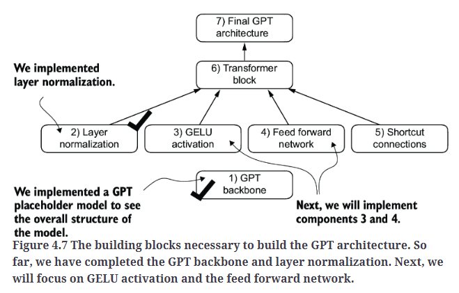
到目前为止,我们已经实现了GPT架构所需的两个基础组件,如Fig4.7所示。
为什么不使用BatchNorm原因:
LLM通常需要大量计算资源,而可用的硬件或具体的应用场景可能会决定训练或推理时的batch size。由于层归一化对每个输入独立归一化,而不依赖batch size,因此在这些场景下提供了更大的灵活性和稳定性。这种特性在分布式训练或资源受限的环境中部署模型时尤为有利。
4.Implementing a feed forward network with GELU activations
在深度学习领域,ReLU激活函数因其简单性和在各种神经网络架构中的有效性,长期以来被广泛使用。然而,在LLM领域,除了传统的ReLU之外,还使用了其他几种激活函数。其中两个值得注意的示例是GELU(Gaussian Error Linear Unit)和SwiGLU(Swish-Gated Linear Unit)。
GELU和SwiGLU是更复杂且更平滑的激活函数。与更简单的ReLU相比,它们能够提升深度学习模型的性能。

1
2
3
4
5
6
7
8
9
10
#An implementation of the GELU activation function
class GELU(nn.Module):
    def __init__(self):
        super().__init__()

    def forward(self, x):
        return 0.5 * x * (1 + torch.tanh(
            torch.sqrt(torch.tensor(2.0 / torch.pi)) *
            (x + 0.044715 * torch.pow(x, 3))
        ))
1
2
3
4
5
6
7
8
9
10
11
12
13
14
15
16
17
18
19
import matplotlib.pyplot as plt

gelu, relu = GELU(), nn.ReLU()

# Some sample data
x = torch.linspace(-3, 3, 100)
y_gelu, y_relu = gelu(x), relu(x)

plt.figure(figsize=(8, 3))
for i, (y, label) in enumerate(zip([y_gelu, y_relu], ["GELU", "ReLU"]), 1):
    plt.subplot(1, 2, i)
    plt.plot(x, y)
    plt.title(f"{label} activation function")
    plt.xlabel("x")
    plt.ylabel(f"{label}(x)")
    plt.grid(True)

plt.tight_layout()
plt.show()

GELU的平滑特性在训练过程中能够带来更好的优化效果,因为它允许对模型参数进行更细微的调整。相比之下,ReLU在零点处存在一个尖角,这有时会使优化变得更加困难,特别是在非常深或结构复杂的网络中。此外,与ReLU不同,后者对于所有负值输入都会输出零,而GELU对负值输入仍会产生一个小的非零输出。这一特性意味着,在训练过程中,即使神经元接收到负值输入,它们仍然可以参与学习过程,尽管贡献会比正值输入较小。
接下来,让我们使用GELU激活函数来实现一个小型神经网络模块FeedForward。
1
2
3
4
5
6
7
8
9
10
11
12
#A feed forward neural network module
class FeedForward(nn.Module):
def __init__(self, cfg):
super().__init__()
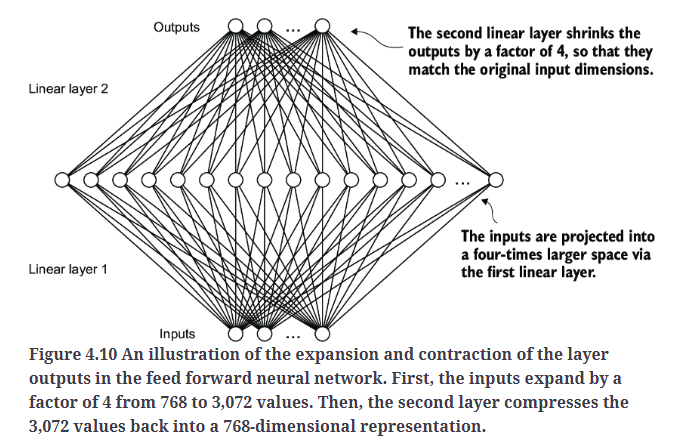
self.layers = nn.Sequential(
nn.Linear(cfg["emb_dim"], 4 * cfg["emb_dim"]),
GELU(),
nn.Linear(4 * cfg["emb_dim"], cfg["emb_dim"]),
)
def forward(self, x):
return self.layers(x)

1
2
3
4
5
6
ffn = FeedForward(GPT_CONFIG_124M)

# input shape: [batch_size, num_token, emb_size]
x = torch.rand(2, 3, 768)
out = ffn(x)
print(out.shape) #torch.Size([2, 3, 768])
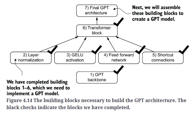
如Fig4.11所示,我们已经实现了LLM的大部分核心构建模块。

5.Adding shortcut connections
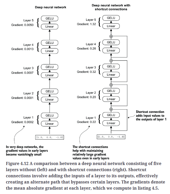
构建Fig4.12所示的网络:
1
2
3
4
5
6
7
8
9
10
11
12
13
14
15
16
17
18
19
20
21
22
23
24
25
26
27
28
29
30
31
32
33
34
35
36
37
38
39
40
41
class ExampleDeepNeuralNetwork(nn.Module):
    def __init__(self, layer_sizes, use_shortcut):
        super().__init__()
        self.use_shortcut = use_shortcut
        self.layers = nn.ModuleList([
            nn.Sequential(nn.Linear(layer_sizes[0], layer_sizes[1]), GELU()),
            nn.Sequential(nn.Linear(layer_sizes[1], layer_sizes[2]), GELU()),
            nn.Sequential(nn.Linear(layer_sizes[2], layer_sizes[3]), GELU()),
            nn.Sequential(nn.Linear(layer_sizes[3], layer_sizes[4]), GELU()),
            nn.Sequential(nn.Linear(layer_sizes[4], layer_sizes[5]), GELU())
        ])

    def forward(self, x):
        for layer in self.layers:
            # Compute the output of the current layer
            layer_output = layer(x)
            # Check if shortcut can be applied
            if self.use_shortcut and x.shape == layer_output.shape:
                x = x + layer_output
            else:
                x = layer_output
        return x


def print_gradients(model, x):
    # Forward pass
    output = model(x) #模型执行前向传播
    target = torch.tensor([[0.]])

    # Calculate loss based on how close the target
    # and output are
    loss = nn.MSELoss()
    loss = loss(output, target)

    # Backward pass to calculate the gradients
    loss.backward()

    for name, param in model.named_parameters():
        if 'weight' in name:
            # Print the mean absolute gradient of the weights
            print(f"{name} has gradient mean of {param.grad.abs().mean().item()}")
.named_parameters()返回模型中所有可训练参数的名称和参数张量。我们可以通过model.named_parameters()遍历所有权重参数。假设某一层的权重参数是一个$3 \times 3$矩阵,那么该层将有$3 \times 3$个梯度值。我们计算这些梯度值的平均绝对值,从而为该层生成一个单一的梯度值,以便更容易比较不同层之间的梯度大小。
没有残差连接时的梯度:
1
2
3
4
5
6
7
8
9
layer_sizes = [3, 3, 3, 3, 3, 1]

sample_input = torch.tensor([[1., 0., -1.]])

torch.manual_seed(123)
model_without_shortcut = ExampleDeepNeuralNetwork(
    layer_sizes, use_shortcut=False
)
print_gradients(model_without_shortcut, sample_input)
输出为:
1
2
3
4
5
layers.0.0.weight has gradient mean of 0.00020173587836325169
layers.1.0.weight has gradient mean of 0.0001201116101583466
layers.2.0.weight has gradient mean of 0.0007152041653171182
layers.3.0.weight has gradient mean of 0.001398873864673078
layers.4.0.weight has gradient mean of 0.005049646366387606
从上述输出可以看出,梯度在从最后一层layers.4向第一层layers.0传播的过程中逐渐变小,这一现象被称为梯度消失问题。
使用残差连接时的梯度:
1
2
3
4
5
torch.manual_seed(123)
model_with_shortcut = ExampleDeepNeuralNetwork(
    layer_sizes, use_shortcut=True
)
print_gradients(model_with_shortcut, sample_input)
输出为:
1
2
3
4
5
layers.0.0.weight has gradient mean of 0.2216978669166565
layers.1.0.weight has gradient mean of 0.20694100856781006
layers.2.0.weight has gradient mean of 0.3289698660373688
layers.3.0.weight has gradient mean of 0.2665731906890869
layers.4.0.weight has gradient mean of 1.3258538246154785
最后一层layers.4的梯度仍然比其他层大。然而,随着梯度向第一层layers.0传播,其值逐渐稳定,并不会缩小到极小的程度。
6.Connecting attention and linear layers in a transformer block
transformer block:

代码实现:
1
2
3
4
5
6
7
8
9
10
11
12
13
14
15
16
17
18
19
20
21
22
23
24
25
26
27
28
29
30
31
32
33
34
35
#The transformer block component of GPT
from previous_chapters import MultiHeadAttention


class TransformerBlock(nn.Module):
    def __init__(self, cfg):
        super().__init__()
        self.att = MultiHeadAttention(
            d_in=cfg["emb_dim"],
            d_out=cfg["emb_dim"],
            context_length=cfg["context_length"],
            num_heads=cfg["n_heads"],
            dropout=cfg["drop_rate"],
            qkv_bias=cfg["qkv_bias"])
        self.ff = FeedForward(cfg)
        self.norm1 = LayerNorm(cfg["emb_dim"])
        self.norm2 = LayerNorm(cfg["emb_dim"])
        self.drop_shortcut = nn.Dropout(cfg["drop_rate"])

    def forward(self, x):
        # Shortcut connection for attention block
        shortcut = x
        x = self.norm1(x)
        x = self.att(x)  # Shape [batch_size, num_tokens, emb_size]
        x = self.drop_shortcut(x)
        x = x + shortcut  # Add the original input back

        # Shortcut connection for feed forward block
        shortcut = x
        x = self.norm2(x)
        x = self.ff(x)
        x = self.drop_shortcut(x)
        x = x + shortcut  # Add the original input back

        return x
层归一化在多头注意力和前馈网络之前应用,这称之为Pre-LayerNorm。在较早的架构(如原始transformer模型)中,在自注意力和前馈网络之后才应用层归一化,这种方法称之为Post-LayerNorm,但通常会导致较差的训练动态。
1
2
3
4
5
6
7
8
torch.manual_seed(123)

x = torch.rand(2, 4, 768)  # Shape: [batch_size, num_tokens, emb_dim]
block = TransformerBlock(GPT_CONFIG_124M)
output = block(x)

print("Input shape:", x.shape) #Input shape: torch.Size([2, 4, 768])
print("Output shape:", output.shape) #Output shape: torch.Size([2, 4, 768])
7.Coding the GPT model
GPT-2模型的整体结构如Fig4.15所示。在1.24亿参数的GPT-2模型中,transformer block被重复12次。在最大规模的GPT-2模型(15.42亿参数)中,transformer block被重复48次。

实现代码为:
1
2
3
4
5
6
7
8
9
10
11
12
13
14
15
16
17
18
19
20
21
22
23
24
25
26
27
28
29
30
31
32
33
34
#The GPT model architecture implementation
class GPTModel(nn.Module):
    def __init__(self, cfg):
        super().__init__()
        self.tok_emb = nn.Embedding(cfg["vocab_size"], cfg["emb_dim"])
        self.pos_emb = nn.Embedding(cfg["context_length"], cfg["emb_dim"])
        self.drop_emb = nn.Dropout(cfg["drop_rate"])

        self.trf_blocks = nn.Sequential(
            *[TransformerBlock(cfg) for _ in range(cfg["n_layers"])])

        self.final_norm = LayerNorm(cfg["emb_dim"])
        self.out_head = nn.Linear(
            cfg["emb_dim"], cfg["vocab_size"], bias=False
        )

    def forward(self, in_idx):
        batch_size, seq_len = in_idx.shape
        tok_embeds = self.tok_emb(in_idx)
        pos_embeds = self.pos_emb(torch.arange(seq_len, device=in_idx.device))
        x = tok_embeds + pos_embeds  # Shape [batch_size, num_tokens, emb_size]
        x = self.drop_emb(x)
        x = self.trf_blocks(x)
        x = self.final_norm(x)
        logits = self.out_head(x)
        return logits

torch.manual_seed(123)
model = GPTModel(GPT_CONFIG_124M)

out = model(batch)
print("Input batch:\n", batch)
print("\nOutput shape:", out.shape)
print(out)
输出为:
1
2
3
4
5
6
7
8
9
10
11
12
13
14
15
Input batch:
 tensor([[6109, 3626, 6100,  345],
        [6109, 1110, 6622,  257]])

Output shape: torch.Size([2, 4, 50257])
tensor([[[ 0.1381,  0.0077, -0.1963,  ..., -0.0222, -0.1060,  0.1717],
         [ 0.3865, -0.8408, -0.6564,  ..., -0.5163,  0.2369, -0.3357],
         [ 0.6989, -0.1829, -0.1631,  ...,  0.1472, -0.6504, -0.0056],
         [-0.4290,  0.1669, -0.1258,  ...,  1.1579,  0.5303, -0.5549]],

        [[ 0.1094, -0.2894, -0.1467,  ..., -0.0557,  0.2911, -0.2824],
         [ 0.0882, -0.3552, -0.3527,  ...,  1.2930,  0.0053,  0.1898],
         [ 0.6091,  0.4702, -0.4094,  ...,  0.7688,  0.3787, -0.1974],
         [-0.0612, -0.0737,  0.4751,  ...,  1.2463, -0.3834,  0.0609]]],
       grad_fn=<UnsafeViewBackward0>)
计算模型的总参数量:
1
2
total_params = sum(p.numel() for p in model.parameters())
print(f"Total number of parameters: {total_params:,}") #Total number of parameters: 163,009,536
我们之前提到要初始化一个1.24亿参数的GPT模型,那么为什么实际的参数数量是1.63亿呢?
那是因为在原始GPT-2架构中使用了权重共享(weight tying)。详细来说就是,GPT-2在输出层重复使用了token嵌入层的权重。为了更好的理解这一点,让我们查看GPTModel初始化的token嵌入层和线性输出层的张量大小。
1
2
print("Token embedding layer shape:", model.tok_emb.weight.shape)
print("Output layer shape:", model.out_head.weight.shape)
输出为:
1
2
Token embedding layer shape: torch.Size([50257, 768])
Output layer shape: torch.Size([50257, 768])
为了考虑权重共享,让我们从GPT-2的总参数量中减去输出层的参数量,以得到实际独立存储的参数总数。
1
2
total_params_gpt2 =  total_params - sum(p.numel() for p in model.out_head.parameters())
print(f"Number of trainable parameters considering weight tying: {total_params_gpt2:,}")
输出为:
1
Number of trainable parameters considering weight tying: 124,412,160
正如我们所看到的,在去除输出层的重复参数后,模型的总参数量变为1.24亿,这与原始GPT-2模型的大小完全匹配。
权重共享可以减少模型的内存占用和计算复杂度。然而,根据作者经验,使用独立的token嵌入层和输出层可以提升训练效果和模型性能,因此,在我们的GPTModel实现中,我们采用了独立的嵌入层和输出层。这一点在现代LLM中也是如此。
接下来,让我们计算这个1.63亿参数的GPTModel所需的内存大小:
1
2
3
4
5
6
7
# Calculate the total size in bytes (assuming float32, 4 bytes per parameter)
total_size_bytes = total_params * 4

# Convert to megabytes
total_size_mb = total_size_bytes / (1024 * 1024)

print(f"Total size of the model: {total_size_mb:.2f} MB")
输出为:
1
Total size of the model: 621.83 MB
8.Generating text
让我们简要回顾生成式模型(如LLM)如何逐个单词(或token)生成文本的过程。
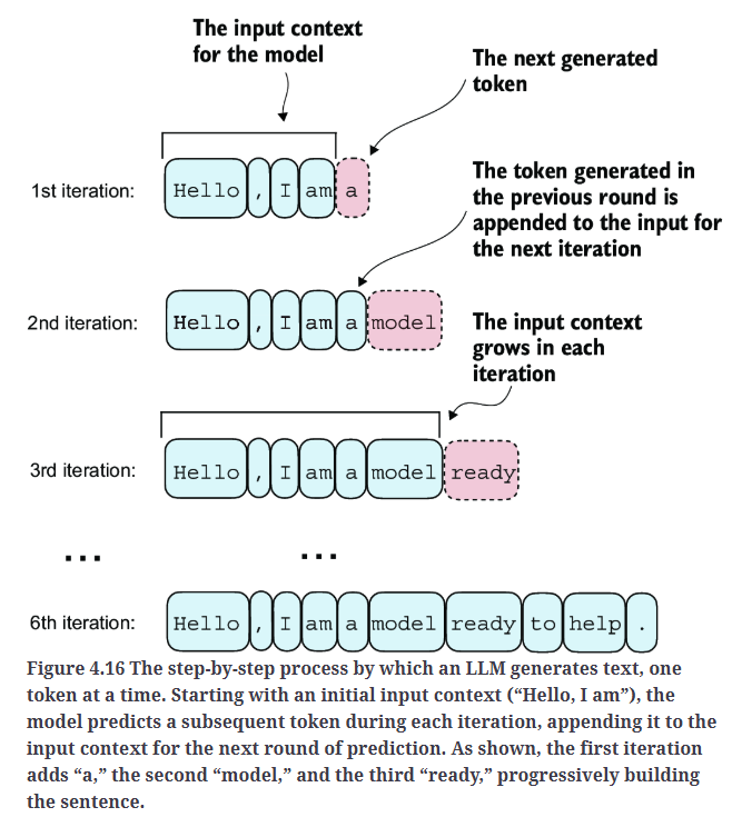
当前的GPTModel输出的是形状为[batch_size, num_token, vocab_size]的张量。那么GPT模型如何从这些输出张量转换为最终生成的文本?
如Fig4.17所示,GPT模型从输出张量转换为生成文本涉及以下几个步骤:

代码实现:
1
2
3
4
5
6
7
8
9
10
11
12
13
14
15
16
17
18
19
20
21
22
23
24
25
26
27
def generate_text_simple(model, idx, max_new_tokens, context_size):
    # idx is (batch, n_tokens) array of indices in the current context
    for _ in range(max_new_tokens):

        # Crop current context if it exceeds the supported context size
        # E.g., if LLM supports only 5 tokens, and the context size is 10
        # then only the last 5 tokens are used as context
        idx_cond = idx[:, -context_size:]

        # Get the predictions
        with torch.no_grad():
            logits = model(idx_cond)

        # Focus only on the last time step
        # (batch, n_tokens, vocab_size) becomes (batch, vocab_size)
        logits = logits[:, -1, :]

        # Apply softmax to get probabilities
        probas = torch.softmax(logits, dim=-1)  # (batch, vocab_size)

        # Get the idx of the vocab entry with the highest probability value
        idx_next = torch.argmax(probas, dim=-1, keepdim=True)  # (batch, 1)

        # Append sampled index to the running sequence
        idx = torch.cat((idx, idx_next), dim=1)  # (batch, n_tokens+1)

    return idx
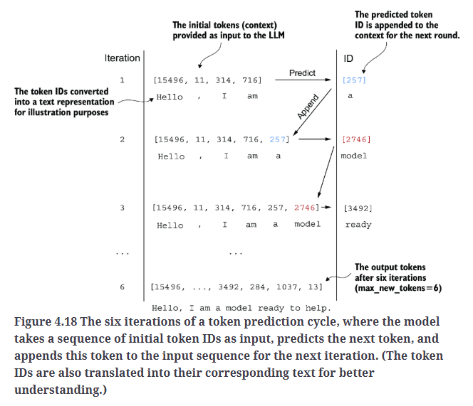
整个过程如Fig4.18所示:
1
2
3
4
5
6
7
8
9
10
11
12
13
14
15
16
17
18
19
20
21
22
start_context = "Hello, I am"

encoded = tokenizer.encode(start_context)
print("encoded:", encoded) #encoded: [15496, 11, 314, 716]

encoded_tensor = torch.tensor(encoded).unsqueeze(0)
print("encoded_tensor.shape:", encoded_tensor.shape) #encoded_tensor.shape: torch.Size([1, 4])

model.eval() # disable dropout

out = generate_text_simple(
    model=model,
    idx=encoded_tensor,
    max_new_tokens=6,
    context_size=GPT_CONFIG_124M["context_length"]
)

print("Output:", out) #Output: tensor([[15496,    11,   314,   716, 27018, 24086, 47843, 30961, 42348,  7267]])
print("Output length:", len(out[0])) #Output length: 10

decoded_text = tokenizer.decode(out.squeeze(0).tolist())
print(decoded_text) #Hello, I am Featureiman Byeswickattribute argue
上述代码中,模型并未生成连贯的文本,这是因为我们尚未对其进行训练,其权重仍然是随机初始化的。