本文为原创文章,未经本人允许,禁止转载。转载请注明出处。
1.使用sklearn建立决策树
1
2
3
4
5
6
7
8
9
from sklearn.datasets import load_iris
from sklearn import tree

iris = load_iris()
clf = tree.DecisionTreeClassifier()
clf = clf.fit(iris.data, iris.target)

# 产生预测结果
predicted = clf.predict(iris.data)
DecisionTreeClassifier中部分参数解释:
criterion:决策树划分标准。默认为“gini”。max_depth:限制树的深度。
iris数据集概览print(iris.DESCR):
1
2
3
4
5
6
7
8
9
10
11
12
13
14
15
16
17
18
19
20
21
22
23
24
25
26
27
28
29
30
31
32
33
34
35
36
37
38
39
40
41
42
43
44
45
46
47
48
49
50
51
52
53
54
55
56
57
58
59
60
61
62
Iris Plants Database
====================

Notes
-----
Data Set Characteristics:
    :Number of Instances: 150 (50 in each of three classes)
    :Number of Attributes: 4 numeric, predictive attributes and the class
    :Attribute Information:
        - sepal length in cm
        - sepal width in cm
        - petal length in cm
        - petal width in cm
        - class:
                - Iris-Setosa
                - Iris-Versicolour
                - Iris-Virginica
    :Summary Statistics:

    ============== ==== ==== ======= ===== ====================
                    Min  Max   Mean    SD   Class Correlation
    ============== ==== ==== ======= ===== ====================
    sepal length:   4.3  7.9   5.84   0.83    0.7826
    sepal width:    2.0  4.4   3.05   0.43   -0.4194
    petal length:   1.0  6.9   3.76   1.76    0.9490  (high!)
    petal width:    0.1  2.5   1.20  0.76     0.9565  (high!)
    ============== ==== ==== ======= ===== ====================

    :Missing Attribute Values: None
    :Class Distribution: 33.3% for each of 3 classes.
    :Creator: R.A. Fisher
    :Donor: Michael Marshall (MARSHALL%PLU@io.arc.nasa.gov)
    :Date: July, 1988

This is a copy of UCI ML iris datasets.
http://archive.ics.uci.edu/ml/datasets/Iris

The famous Iris database, first used by Sir R.A Fisher

This is perhaps the best known database to be found in the
pattern recognition literature.  Fisher's paper is a classic in the field and
is referenced frequently to this day.  (See Duda & Hart, for example.)  The
data set contains 3 classes of 50 instances each, where each class refers to a
type of iris plant.  One class is linearly separable from the other 2; the
latter are NOT linearly separable from each other.

References
----------
   - Fisher,R.A. "The use of multiple measurements in taxonomic problems"
     Annual Eugenics, 7, Part II, 179-188 (1936); also in "Contributions to
     Mathematical Statistics" (John Wiley, NY, 1950).
   - Duda,R.O., & Hart,P.E. (1973) Pattern Classification and Scene Analysis.
     (Q327.D83) John Wiley & Sons.  ISBN 0-471-22361-1.  See page 218.
   - Dasarathy, B.V. (1980) "Nosing Around the Neighborhood: A New System
     Structure and Classification Rule for Recognition in Partially Exposed
     Environments".  IEEE Transactions on Pattern Analysis and Machine
     Intelligence, Vol. PAMI-2, No. 1, 67-71.
   - Gates, G.W. (1972) "The Reduced Nearest Neighbor Rule".  IEEE Transactions
     on Information Theory, May 1972, 431-433.
   - See also: 1988 MLC Proceedings, 54-64.  Cheeseman et al"s AUTOCLASS II
     conceptual clustering system finds 3 classes in the data.
   - Many, many more ...
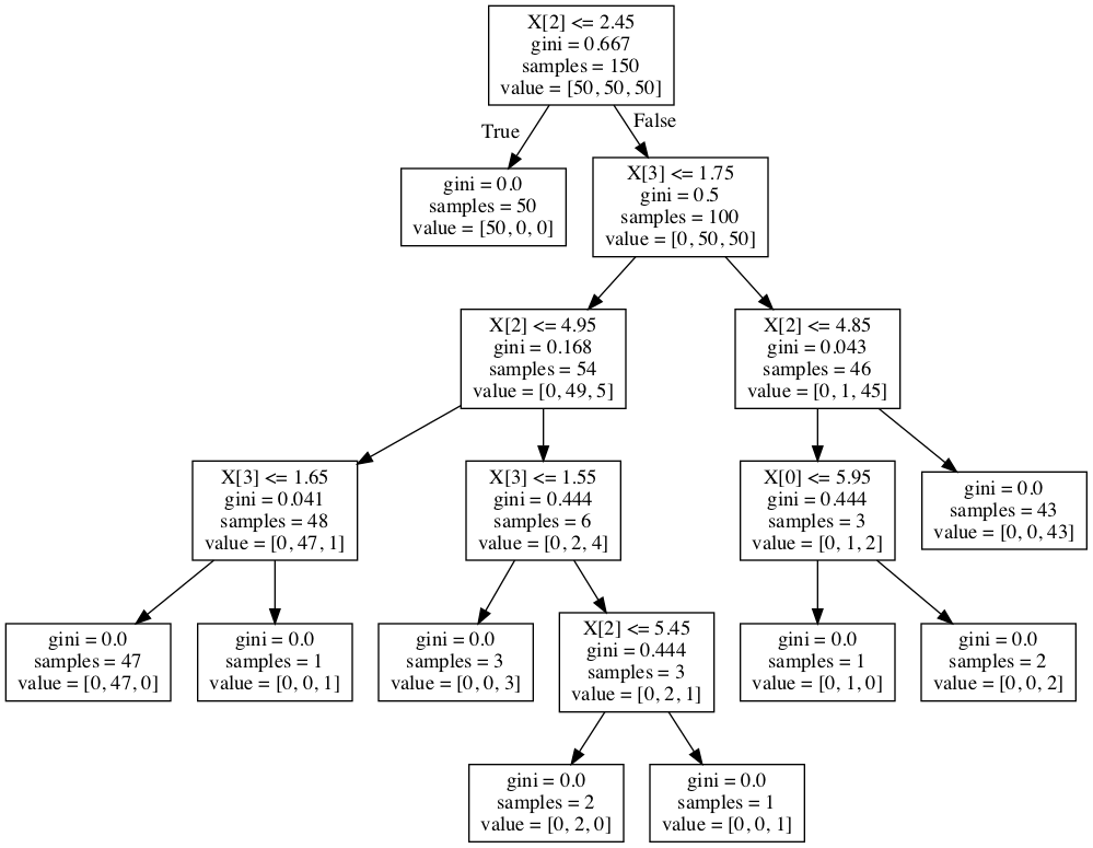
2.将分类结果显示在图上
1
2
3
4
# 绘制成树形图
from sklearn import tree

tree.export_graphviz(clf, out_file='tree.dot')
使用graphviz读取dot文件并将其转换为png图像进行可视化:dot -Tpng tree.dot -o tree.png。也可转换成svg格式:dot -Tsvg tree.dot -o tree.svg。
graphviz官网:http://www.graphviz.org。
Mac推荐使用homebrew下载graphviz:
brew install graphviz。
3.建立决策边界
首先和第1部分一样,构建决策树分类模型:
1
2
3
4
5
6
7
8
9
10
11
12
13
14
from itertools import product
import numpy as np
import matplotlib.pyplot as plt
from sklearn.datasets import load_iris
from sklearn import tree
iris = load_iris()
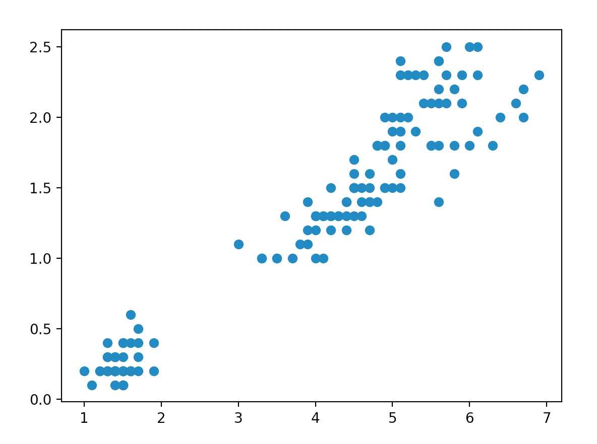
X = iris.data[:, [2, 3]]#只使用两个变量
y = iris.target
clf = tree.DecisionTreeClassifier(max_depth=2)
clf.fit(X, y)
看下X这两个变量的分布情况:
1
2
3
plt.plot()
plt.scatter(X[:, 0], X[:, 1])
plt.show()
绘制决策边界:
1
2
3
4
5
6
7
8
9
10
11
12
13
14
15
16
17
18
x_min, x_max = X[:, 0].min() - 1, X[:, 0].max() + 1
y_min, y_max = X[:, 1].min() - 1, X[:, 1].max() + 1
xx, yy = np.meshgrid(np.arange(x_min, x_max, 0.1), np.arange(y_min, y_max, 0.1))

plt.plot()
Z = clf.predict(np.c_[xx.ravel(), yy.ravel()])
Z = Z.reshape(xx.shape)
#参数alpha为透明度
#参数cmap为colormap
plt.contourf(xx, yy, Z, alpha=0.4, cmap=plt.cm.rainbow)
#参数c为颜色
#参数alpha为透明度
#参数cmap为colormap
plt.scatter(X[:, 0], X[:, 1], c=y, alpha=1, cmap=plt.cm.YlOrRd)
plt.title('Decision Tree')
plt.xlabel('Petal.Length')
plt.ylabel('Petal.Width')
plt.show()
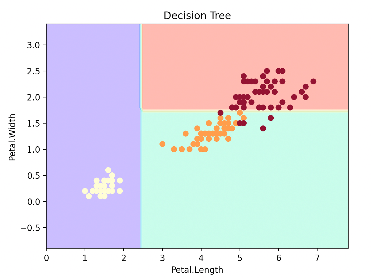
每种底色代表一个类别标签。底色通过plt.contourf绘制。
3.1.numpy.arange
numpy.arange(start,stop,step):
1
2
3
np.arange(0,1,0.2)
#输出为:
#array([0. , 0.2, 0.4, 0.6, 0.8])
3.2.numpy.meshgrid
1
xx,yy=np.meshgrid(np.arange(0,1,0.2),np.arange(1,3,1))
xx为:
1
2
array([[0. , 0.2, 0.4, 0.6, 0.8],
       [0. , 0.2, 0.4, 0.6, 0.8]])
yy为:
1
2
array([[1, 1, 1, 1, 1],
       [2, 2, 2, 2, 2]])
3.3.ravel
1
a = np.arange(12).reshape(3,4)
a为:
1
2
3
array([[ 0,  1,  2,  3],
       [ 4,  5,  6,  7],
       [ 8,  9, 10, 11]])
a.ravel()为扁平化操作:
1
array([ 0,  1,  2,  3,  4,  5,  6,  7,  8,  9, 10, 11])
和a.flatten()的结果是一样的。
3.4.numpy.c_
numpy.c_为按列连接两个矩阵。numpy.r_为按行连接两个矩阵。
1
2
3
4
#1
np.c_[np.array([1,2,3]), np.array([4,5,6])]
#2
np.r_[np.array([1,2,3]), np.array([4,5,6])]
1
2
3
4
5
6
#1
array([[1, 4],
       [2, 5],
       [3, 6]])
#2
array([1, 2, 3, 4, 5, 6])