本文为原创文章,未经本人允许,禁止转载。转载请注明出处。
1.scikit-learn简介
scikit-learn是针对python编程语言的免费软件机器学习库。官网:https://scikit-learn.org/stable/。
2.回归模型
读入待处理数据:
1
2
3
4
import pandas as pd

df = pd.read_csv('salary.csv', index_col=0)#第0列作为index
print(df.head())
1
2
3
4
5
6
   year  salary
1   2.4    6600
2   5.5   10100
3   3.3    7300
4   0.2    5000
5   1.5    6100
数据可视化:
1
2
3
4
5
6
X = df[['year']]#X格式为DataFrame
Y = df['salary'].values#Y格式为ndarray
plt.scatter(X, Y, color='black')
plt.xlabel('year')
plt.ylabel('salary')
plt.show()
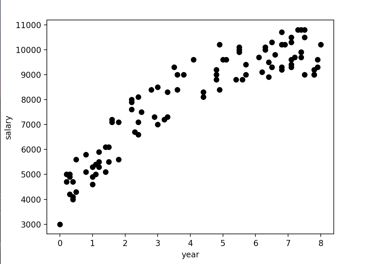
X = df['year']得到的为Series,而X = df[['year']]得到的为DataFrame。X = df['year'].values得到的为ndarray。
构建回归模型:
1
2
3
4
5
from sklearn.linear_model import LinearRegression
regr = LinearRegression()
regr.fit(X, Y)
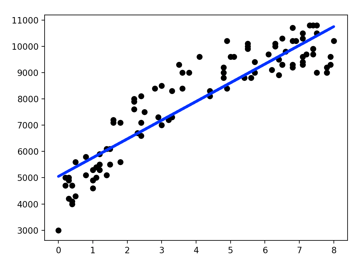
print('Coefficients:', regr.coef_)#Coefficients: [712.59413615]
print('Intercept:', regr.intercept_)#Intercept: 5049.009899813836
将回归线绘制在图上:
1
2
3
plt.scatter(X, Y, color='black')
plt.plot(X, regr.predict(X), color='blue', linewidth=3)
plt.show()
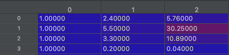
3.多项式线性回归
还是用第2部分的数据,假设我们想构建的模型为:$y=\beta_2 x^2 + \beta_1 x + \beta_0$。
1
2
3
4
5
6
7
8
9
10
from sklearn.linear_model import LinearRegression
from sklearn.preprocessing import PolynomialFeatures

#下面两句用来生成高次项
#degree=2生成:x^0,x^1,x^2
poly_reg = PolynomialFeatures(degree=2)
X_ = poly_reg.fit_transform(X)

regr = LinearRegression()
regr.fit(X_, Y)
X_里存的数据(部分):
绘制回归曲线:
1
2
3
4
5
6
X2 = X.sort_values(['year'])
X2_ = poly_reg.fit_transform(X2)

plt.scatter(X, Y, color='black')
plt.plot(X2, regr.predict(X2_), linewidth=3, color="blue")
plt.show()
因为plt.plot()是逐个点按顺序连接从而绘制曲线的,所以事先需要对$X$进行排序:

4.多元线性回归
以预测房价为例。首先读入房屋数据:
1
2
3
4
import pandas as pd

df = pd.read_csv("house-prices.csv")
print(df.head())
1
2
3
4
5
6
   Home   Price  SqFt      ...       Offers  Brick  Neighborhood
0     1  114300  1790      ...            2     No          East
1     2  114200  2030      ...            3     No          East
2     3  114800  1740      ...            1     No          East
3     4   94700  1980      ...            3     No          East
4     5  119800  2130      ...            3     No          East
将“Brick”列和“Neighborhood”转换成one-hot编码:
get_dummies用法请见:链接。
1
2
house = pd.concat([df,pd.get_dummies(df['Brick']),pd.get_dummies(df['Neighborhood'])],axis=1)
print(house.head())
1
2
3
4
5
6
   Home   Price  SqFt  Bedrooms  Bathrooms  ...   No Yes East  North  West
0     1  114300  1790         2          2  ...    1   0    1      0     0
1     2  114200  2030         4          2  ...    1   0    1      0     0
2     3  114800  1740         3          2  ...    1   0    1      0     0
3     4   94700  1980         3          2  ...    1   0    1      0     0
4     5  119800  2130         3          3  ...    1   0    1      0     0
列“Yes”和列“No”是由列“Brick”分化来的,具有很强的相关性,所以在后续使用时需删除列“Brick”以及列“Yes”和列“No”中的其中一列。同理,列“East”,列“North”和列“West”也具有很强的相关性,也需要删除其中一列:
1
2
3
4
5
6
del house['No']
del house['West']
del house['Brick']
del house['Neighborhood']
del house['Home']#index列也没有意义,需删除
print(house.head())
1
2
3
4
5
6
    Price  SqFt  Bedrooms  Bathrooms  Offers  Yes  East  North
0  114300  1790         2          2       2    0     1      0
1  114200  2030         4          2       3    0     1      0
2  114800  1740         3          2       1    0     1      0
3   94700  1980         3          2       3    0     1      0
4  119800  2130         3          3       3    0     1      0
建立回归模型:
1
2
3
4
5
6
7
from sklearn.linear_model import LinearRegression

regr = LinearRegression()
X = house[["SqFt", "Bedrooms", "Bathrooms", "Offers", "Yes", "East", "North"]]
Y = house["Price"].values
regr.fit(X, Y)
regr.predict(X)
5.回归模型评估
使用第4部分处理过的房价数据。
1
2
3
4
5
import statsmodels.api as sm
X2 = sm.add_constant(X)
est = sm.OLS(Y, X2)
est2 = est.fit()
print(est2.summary())
1
2
3
4
5
6
7
8
9
10
11
12
13
14
15
16
17
18
19
20
21
22
23
24
25
26
27
28
29
30
31
32
33
                            OLS Regression Results
==============================================================================
Dep. Variable:                      y   R-squared:                       0.869
Model:                            OLS   Adj. R-squared:                  0.861
Method:                 Least Squares   F-statistic:                     113.3
Date:                Thu, 16 Sep 2021   Prob (F-statistic):           8.25e-50
Time:                        20:04:24   Log-Likelihood:                -1356.7
No. Observations:                 128   AIC:                             2729.
Df Residuals:                     120   BIC:                             2752.
Df Model:                           7
Covariance Type:            nonrobust
==============================================================================
                 coef    std err          t      P>|t|      [0.025      0.975]
------------------------------------------------------------------------------
const       2.284e+04   1.02e+04      2.231      0.028    2573.371    4.31e+04
SqFt          52.9937      5.734      9.242      0.000      41.640      64.347
Bedrooms    4246.7939   1597.911      2.658      0.009    1083.042    7410.546
Bathrooms   7883.2785   2117.035      3.724      0.000    3691.696    1.21e+04
Offers     -8267.4883   1084.777     -7.621      0.000   -1.04e+04   -6119.706
Yes          1.73e+04   1981.616      8.729      0.000    1.34e+04    2.12e+04
East       -2.224e+04   2531.758     -8.785      0.000   -2.73e+04   -1.72e+04
North      -2.068e+04   3148.954     -6.568      0.000   -2.69e+04   -1.44e+04
==============================================================================
Omnibus:                        3.026   Durbin-Watson:                   1.921
Prob(Omnibus):                  0.220   Jarque-Bera (JB):                2.483
Skew:                           0.268   Prob(JB):                        0.289
Kurtosis:                       3.421   Cond. No.                     2.38e+04
==============================================================================

Warnings:
[1] Standard Errors assume that the covariance matrix of the errors is correctly specified.
[2] The condition number is large, 2.38e+04. This might indicate that there are
strong multicollinearity or other numerical problems.
OLS为“Ordinary least squares”,即“普通最小二乘法”。
5.1.t检验
summary中有一列t值,即单样本t检验的结果(从数据集中多次随机采样子集用于训练模型,一个自变量便可得到多个coef,从而进行单样本t检验)。$H_0$为$coef=0$,即该自变量与因变量无关。假设当$P<0.05$时拒绝$H_0$,则上述例子中所有自变量均与因变量存在关系。
5.2.F检验
F检验的结果见“F-statistic”和“Prob (F-statistic)”。
\[H_0:\beta_1=\beta_2=\beta_3=...=\beta_k=0\] \[H_1: at \ least \ one \ \beta_k \neq 0\]此处使用的应该是完全随机设计资料的方差分析。
5.3.R-squared
“R-squared”(即$R^2$)指的是线性回归的拟合优度(Goodness of Fit)。$R^2$最大值为1。$R^2$的值越接近1,说明回归直线对观测值的拟合程度越好;反之,$R^2$的值越小,说明回归直线对观测值的拟合程度越差。
\[R^2 = \frac{SSR}{SST}= 1- \frac{SSE}{SST}\]- SSR:回归平方和,Sum of Squares for Regression。
- SSE:残差平方和,Sum of Squares for Error。
- SST:总离差平方和,Sum of Squares for Total。
其中,SST=SSR+SSE。
\[SSE=\sum^n_{i=1}(y_i - \hat{y_i})^2\] \[SST=\sum^n_{i=1}(y_i-y_{avg})^2\]其中,$y_i$为观测值,$\hat{y_i}$为预测值,$y_{avg}$为所有观测值的平均值。
5.3.1.Adjusted R Square
变量越多,虽然会增加过拟合的风险,但是会降低SSE,即增加$R^2$,所以其偏向于变量多的模型(即更复杂的模型)。而Adjusted R Square(“Adj. R-squared”)就是相当于给变量的个数(即模型的复杂程度)加惩罚项。换句话说,如果两个模型,样本数一样,$R^2$一样,那么从Adjusted R Square的角度看,使用变量个数少的那个模型更优。使用Adjusted R Square也算一种奥卡姆剃刀的实例。
\[R^2_{adj}=1-\frac{(n-1)(1-R^2)}{n-p-1}\]其中,$n$是样本数量,$p$是模型中变量的个数。
如果单变量线性回归,则使用$R^2$评估,多变量,则使用Adjusted R Squared。在单变量线性回归中,$R^2$和Adjusted R Squared是一致的。
另外,如果增加更多无意义的变量,则$R^2$和Adjusted R Squared之间的差距会越来越大,Adjusted R Squared会下降。但是如果加入的特征值是显著的,则Adjusted R Squared也会上升。
5.4.AIC和BIC
5.4.1.AIC
AIC:即Akaike Information Criterion,赤池信息准则。是衡量统计模型拟合优良性(Goodness of fit)的一种标准。由于它为日本统计学家赤池弘次创立和发展的,因此又称赤池信息量准则。它建立在熵的概念基础上,可以权衡所估计模型的复杂度和此模型拟合数据的优良性。通常情况下,AIC可定义为:
\[AIC=2k-2\ln (L)\]其中,$k$是参数数量,$n$为样本数,$L$是似然函数。
AIC鼓励数据拟合的优良性但是尽量避免出现过度拟合的情况。所以优先考虑的模型应是AIC值最小的那一个。AIC是寻找可以最好地解释数据但包含最少自由参数的模型。
此处,我们使用的AIC公式具体为:
\[AIC=2k+n\ln (SSE/n)\]SSE的定义及计算见第5.3部分。
5.4.2.BIC
BIC:即Bayesian Information Criterion,贝叶斯信息准则。通常情况下,BIC可定义为:
\[BIC=k\ln (n)-2\ln (L)\]其中,$k$是参数数量,$n$为样本数,$L$是似然函数。
训练模型时,增加参数数量,也就是增加模型复杂度,会增大似然函数,但是也会导致过拟合现象。$k\ln(n)$惩罚项在样本数量较多的情况下可有效防止模型精度过高造成模型复杂度过高的问题,避免维度灾难现象。
AIC公式和BIC公式后半部分是一样的,前半部分是惩罚项,$n$较大时,$k\ln(n) \geqslant 2k$,所以,BIC相比AIC在大数据量时对模型参数惩罚得更多,导致BIC更倾向于选择参数少的简单模型。
5.4.3.根据AIC选择最优模型
1
2
3
4
5
6
7
8
9
10
11
12
13
14
15
16
import itertools

predictorcols = ["SqFt", "Bedrooms", "Bathrooms", "Offers", "Yes", "East", "North"]
AICs = {}
for k in range(1, len(predictorcols) + 1):
    for variables in itertools.combinations(predictorcols, k):
        predictors = X[list(variables)]
        predictors2 = sm.add_constant(predictors)
        est = sm.OLS(Y, predictors2)
        res = est.fit()
        AICs[variables] = res.aic

from collections import Counter

c = Counter(AICs)
c.most_common()[::-10] #选取AIC最小的10种组合
1
2
3
4
5
6
7
8
9
10
11
12
13
14
15
16
#AIC最小的10种组合:
[
(('SqFt', 'Bedrooms', 'Bathrooms', 'Offers', 'Yes', 'East', 'North'), 2729.3189814012494),
(('SqFt', 'Bedrooms', 'Bathrooms', 'Offers', 'Yes'), 2789.5148143560264),
(('SqFt', 'Offers', 'East', 'North'), 2805.929045591597),
(('SqFt', 'Bedrooms', 'Bathrooms', 'East', 'North'), 2827.1498026886024),
(('Bedrooms', 'Bathrooms', 'Offers', 'Yes', 'East'), 2837.9283737790706),
(('Bedrooms', 'Bathrooms', 'Offers', 'Yes'), 2845.973295559599),
(('SqFt', 'Offers'), 2865.6942475349356),
(('Bedrooms', 'Bathrooms', 'Offers', 'East'), 2874.0450207228523),
(('Bedrooms', 'Bathrooms', 'Yes'), 2883.9535408052025),
(('SqFt', 'Yes'), 2896.9093592727936),
(('Bedrooms', 'North'), 2908.6992372764653),
(('Bedrooms', 'Bathrooms'), 2916.035689947397),
(('Bathrooms',), 2936.1658574541634)
]
可以看出AIC最小的模型(即最优的模型)使用了所有的变量。其中,itertools.combinations(predictorcols, k)表示从“predictorcols”任选k个的所有可能组合。例如:
1
2
for variables in itertools.combinations(predictorcols, 2):
    print(variables)
1
2
3
4
5
6
7
8
9
10
11
12
13
14
15
16
17
18
19
20
21
('SqFt', 'Bedrooms')
('SqFt', 'Bathrooms')
('SqFt', 'Offers')
('SqFt', 'Yes')
('SqFt', 'East')
('SqFt', 'North')
('Bedrooms', 'Bathrooms')
('Bedrooms', 'Offers')
('Bedrooms', 'Yes')
('Bedrooms', 'East')
('Bedrooms', 'North')
('Bathrooms', 'Offers')
('Bathrooms', 'Yes')
('Bathrooms', 'East')
('Bathrooms', 'North')
('Offers', 'Yes')
('Offers', 'East')
('Offers', 'North')
('Yes', 'East')
('Yes', 'North')
('East', 'North')
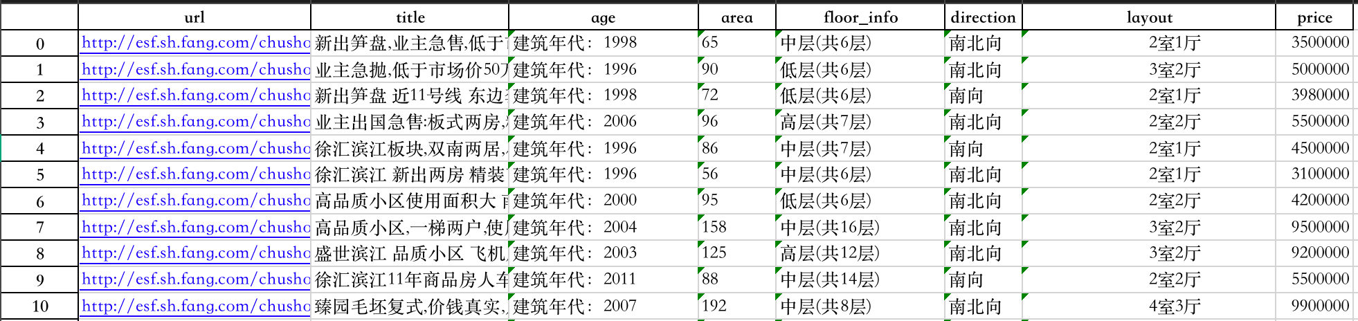
6.实战:使用回归模型分析房屋价格
6.1.读入数据
1
2
3
4
import pandas as pd

df = pd.read_excel("house_price_regression.xlsx")
print(df.head(10))
6.2.资料预处理
1
2
3
4
5
6
7
8
9
10
11
12
13
14
15
16
17
18
df["age"] = df["age"].map(lambda e: 2021 - int(e.strip().strip('建筑年代:'))) # 'age'列改为距今多少年
df[['room', 'living_room']] = df['layout'].str.extract('(\d+)室(\d+)厅')  # 抽取"室"和"厅"的数量
df['room'] = df['room'].astype(int)
df['living_room'] = df['living_room'].astype(int)
df['total_floor'] = df['floor_info'].str.extract('共(\d+)层')  # 提取总楼层数
df['total_floor'] = df['total_floor'].astype(int)
df['floor'] = df['floor_info'].str.extract('^(.)层')  # 抽取"高、中、低"层
df['direction'] = df['direction'].map(lambda e: e.strip())
del df['layout']
del df['floor_info']
del df['title']
del df['url']
df = pd.concat([df, pd.get_dummies(df['direction']), pd.get_dummies(df['floor'])], axis=1)  # 创建哑变量
del df['南北向']
del df['低']
del df['direction']
del df['floor']
print(df.head())
1
2
3
4
5
6
   age  area    price  room  living_room  total_floor ...  东向  南向  西南向  西向  中  高
0   23    65  3500000     2            1            6 ...   0   0    0   0  1  0
1   25    90  5000000     3            2            6 ...   0   0    0   0  0  0
2   23    72  3980000     2            1            6 ...   0   1    0   0  0  0
3   15    96  5500000     2            2            7 ...   0   0    0   0  0  1
4   25    86  4500000     2            1            7 ...   0   1    0   0  1  0
map用法见:map。- 正则表达式的用法见:正则表达式。
pandas.concat的用法见:pandas.concat。pandas.get_dummies的用法见:pandas.get_dummies。
Series.str.extract()以字符串形式访问Series并提取正则表达式。pandas.Series.astype用于类型转换。
6.3.回归模型
绘制散点图:
1
2
3
4
5
6
7
import matplotlib

matplotlib.use('TkAgg')
import matplotlib.pyplot as plt

df[['price', 'area']].plot(kind='scatter', x='area', y='price', figsize=[10, 5])
plt.show()
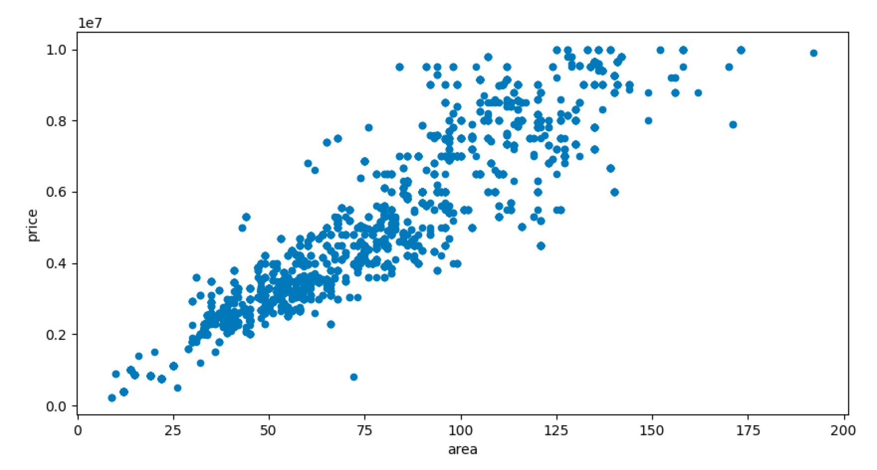
建立一个一元回归模型,房屋大小和价格的关系:
1
2
3
4
5
6
7
8
9
from sklearn.linear_model import LinearRegression
import numpy as np

y = np.array(df['price']).reshape(-1, 1)
X = np.array(df['area']).reshape(-1, 1)
regr = LinearRegression()
regr.fit(X, y)
print('Coefficient:{}'.format(regr.coef_))
print('Intercept:{}'.format(regr.intercept_))
1
2
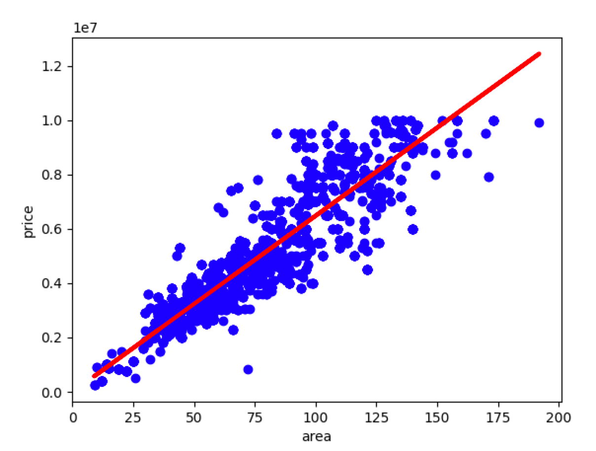
Coefficient:[[64846.01038065]]
Intercept:[-9165.21745733]
format格式化函数见本文第6.5部分。
绘制回归线:
1
2
3
4
5
plt.scatter(X, y, color='blue')
plt.plot(X, regr.predict(X), linewidth=3, color='red')
plt.xlabel('area')
plt.ylabel('price')
plt.show()
建立多元回归模型:
1
2
3
4
y = df['price'].values
X = df[['age', 'area', 'room', 'living_room', 'total_floor', '东南向', '东向', '南向', '西南向', '西向', '中', '高']]
regr = LinearRegression()
regr.fit(X, y)
6.4.评估回归模型
1
2
3
4
5
6
import statsmodels.api as sm

X2 = sm.add_constant(X)
est = sm.OLS(y, X2)
est2 = est.fit()
print(est2.summary())
1
2
3
4
5
6
7
8
9
10
11
12
13
14
15
16
17
18
19
20
21
22
23
24
25
26
27
28
29
30
31
32
33
34
35
36
37
38
                            OLS Regression Results
==============================================================================
Dep. Variable:                      y   R-squared:                       0.850
Model:                            OLS   Adj. R-squared:                  0.850
Method:                 Least Squares   F-statistic:                     1316.
Date:                Tue, 21 Sep 2021   Prob (F-statistic):               0.00
Time:                        18:02:49   Log-Likelihood:                -42322.
No. Observations:                2792   AIC:                         8.467e+04
Df Residuals:                    2779   BIC:                         8.475e+04
Df Model:                          12
Covariance Type:            nonrobust
===============================================================================
                  coef    std err          t      P>|t|      [0.025      0.975]
-------------------------------------------------------------------------------
const        2.061e+05   8.69e+04      2.370      0.018    3.56e+04    3.77e+05
age           116.4043     37.023      3.144      0.002      43.809     189.000
area          6.93e+04   1237.714     55.993      0.000    6.69e+04    7.17e+04
room        -3.412e+05   4.31e+04     -7.922      0.000   -4.26e+05   -2.57e+05
living_room -3.932e+04   5.62e+04     -0.700      0.484   -1.49e+05    7.08e+04
total_floor  1.511e+04   2680.686      5.638      0.000    9857.449    2.04e+04
东南向          5.827e+05   2.51e+05      2.322      0.020    9.07e+04    1.07e+06
东向          -5.275e+05   1.73e+05     -3.054      0.002   -8.66e+05   -1.89e+05
南向            2.09e+05   3.73e+04      5.608      0.000    1.36e+05    2.82e+05
西南向         -1.445e+06   2.07e+05     -6.966      0.000   -1.85e+06   -1.04e+06
西向           8.085e+05   3.13e+05      2.583      0.010    1.95e+05    1.42e+06
中           -2.727e+05   4.84e+04     -5.631      0.000   -3.68e+05   -1.78e+05
高            6.892e+04   5.26e+04      1.310      0.190   -3.43e+04    1.72e+05
==============================================================================
Omnibus:                      182.215   Durbin-Watson:                   1.701
Prob(Omnibus):                  0.000   Jarque-Bera (JB):              552.957
Skew:                           0.311   Prob(JB):                    8.45e-121
Kurtosis:                       5.090   Cond. No.                     9.04e+03
==============================================================================

Notes:
[1] Standard Errors assume that the covariance matrix of the errors is correctly specified.
[2] The condition number is large, 9.04e+03. This might indicate that there are
strong multicollinearity or other numerical problems.
通过AIC选择最佳参数组合:
1
2
3
4
5
6
7
8
9
10
11
12
13
14
15
predictorcols = ['age', 'area', 'room', 'living_room', 'total_floor', '东南向', '东向', '南向', '西南向', '西向', '中', '高']
import itertools

AICs = {}
for k in range(1, len(predictorcols) + 1):
    for variables in itertools.combinations(predictorcols, k):
        predictors = X[list(variables)]
        predictors2 = sm.add_constant(predictors)
        est = sm.OLS(y, predictors2)
        res = est.fit()
        AICs[variables] = res.aic
from collections import Counter

c = Counter(AICs)
print(c.most_common()[::-10])
结果不再展示,类似第5.4.3部分。
6.5.format格式化函数
str.format()的用法见下:
1
2
3
4
5
6
7
8
>>>"{} {}".format("hello", "world")    # 不设置指定位置,按默认顺序
'hello world'

>>> "{0} {1}".format("hello", "world")  # 设置指定位置
'hello world'

>>> "{1} {0} {1}".format("hello", "world")  # 设置指定位置
'world hello world'
也可以设置参数:
1
2
3
4
5
6
7
8
9
print("网站名:{name}, 地址 {url}".format(name="菜鸟教程", url="www.runoob.com"))

# 通过字典设置参数
site = {"name": "菜鸟教程", "url": "www.runoob.com"}
print("网站名:{name}, 地址 {url}".format(**site))

# 通过列表索引设置参数
my_list = ['菜鸟教程', 'www.runoob.com']
print("网站名:{0[0]}, 地址 {0[1]}".format(my_list))  # "0" 是必须的
1
2
3
网站名:菜鸟教程, 地址 www.runoob.com
网站名:菜鸟教程, 地址 www.runoob.com
网站名:菜鸟教程, 地址 www.runoob.com
str.format()格式化数字的多种方法:
| 数字 | 格式 | 输出 | 描述 |
|---|---|---|---|
| 3.1415926 | {:.2f} | 3.14 | 保留小数点后两位 |
| 3.1415926 | {:+.2f} | +3.14 | 带符号保留小数点后两位 |
| -1 | {:+.2f} | -1.00 | 带符号保留小数点后两位 |
| 2.71828 | {:.0f} | 3 | 不带小数 |
| 5 | {:0>2d} | 05 | 数字补零 (填充左边, 宽度为2) |
| 5 | {:x<4d} | 5xxx | 数字补x (填充右边, 宽度为4) |
| 10 | {:x<4d} | 10xx | 数字补x (填充右边, 宽度为4) |
| 1000000 | {:,} | 1,000,000 | 以逗号分隔的数字格式 |
| 0.25 | {:.2%} | 25.00% | 百分比格式 |
| 1000000000 | {:.2e} | 1.00e+09 | 指数记法 |
| 13 | {:>10d} | 13 | 右对齐 (默认, 宽度为10) |
| 13 | {:<10d} | 13 | 左对齐 (宽度为10) |
| 13 | {:^10d} | 13 | 中间对齐 (宽度为10) |
| 11 | '{:b}'.format(11) |
1011 | 二进制 |
| 11 | '{:d}'.format(11) |
11 | 十进制 |
| 11 | '{:o}'.format(11) |
13 | 八进制 |
| 11 | '{:x}'.format(11) |
b | 十六进制 |
| 11 | '{:#x}'.format(11) |
0xb | 进制 |
| 11 | '{:#X}'.format(11) |
0XB | 进制 |
^,<,>分别是居中、左对齐、右对齐,后面带宽度,:号后面带填充的字符,只能是一个字符,不指定则默认是用空格填充。
+表示在正数前显示+,负数前显示-;(空格)表示在正数前加空格。
此外我们可以使用大括号{}来转义大括号,如下实例:
1
2
3
print ("{} 对应的位置是 0".format("runoob"))
#输出为:
#runoob 对应的位置是 {0}