【从零开始构建大语言模型】系列博客为”Build a Large Language Model (From Scratch)”一书的个人读书笔记。
- 原书链接:Build a Large Language Model (From Scratch)。
- 官方示例代码:LLMs-from-scratch。
本文为原创文章,未经本人允许,禁止转载。转载请注明出处。
1.Pretraining on unlabeled data

2.Evaluating generative text models
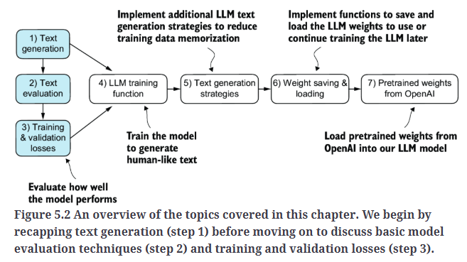
Fig5.2的蓝色模块为本部分将详细介绍的内容。
2.1.Using GPT to generate text
1
2
3
4
5
6
7
8
9
10
11
12
13
14
15
16
import torch
from previous_chapters import GPTModel

GPT_CONFIG_124M = {
    "vocab_size": 50257,   # Vocabulary size
    "context_length": 256, # Shortened context length (orig: 1024)
    "emb_dim": 768,        # Embedding dimension
    "n_heads": 12,         # Number of attention heads
    "n_layers": 12,        # Number of layers
    "drop_rate": 0.1,      # Dropout rate
    "qkv_bias": False      # Query-key-value bias
}

torch.manual_seed(123)
model = GPTModel(GPT_CONFIG_124M)
model.eval();  # Disable dropout during inference
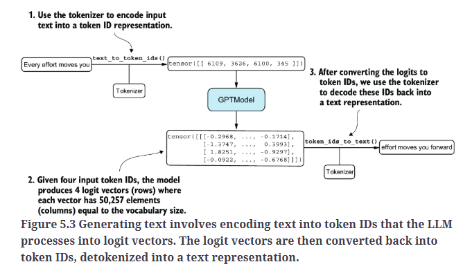
使用GPTModel实例,我们采用第4章中的generate_text_simple函数,并引入了两个实用函数:text_to_token_ids和token_ids_to_text,这两个函数用于在文本和token表示之间进行转换。
1
2
3
4
5
6
7
8
9
10
11
12
13
14
15
16
17
18
19
20
21
22
23
import tiktoken
from previous_chapters import generate_text_simple

def text_to_token_ids(text, tokenizer):
    encoded = tokenizer.encode(text, allowed_special={'<|endoftext|>'})
    encoded_tensor = torch.tensor(encoded).unsqueeze(0) # add batch dimension
    return encoded_tensor

def token_ids_to_text(token_ids, tokenizer):
    flat = token_ids.squeeze(0) # remove batch dimension
    return tokenizer.decode(flat.tolist())

start_context = "Every effort moves you"
tokenizer = tiktoken.get_encoding("gpt2")

token_ids = generate_text_simple(
    model=model,
    idx=text_to_token_ids(start_context, tokenizer),
    max_new_tokens=10,
    context_size=GPT_CONFIG_124M["context_length"]
)

print("Output text:\n", token_ids_to_text(token_ids, tokenizer))
输出为:
1
2
Output text:
 Every effort moves you rentingetic wasnم refres RexMeCHicular stren
2.2.Calculating the text generation loss
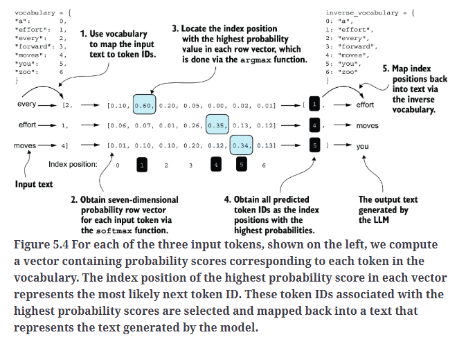
Fig5.4展示了LLM生成文本的5个步骤。
1
2
3
4
5
6
7
8
9
10
11
12
13
14
15
16
17
18
19
20
21
22
23
24
25
26
27
28
29
30
31
inputs = torch.tensor([[16833, 3626, 6100],   # ["every effort moves",
                       [40,    1107, 588]])   #  "I really like"]

targets = torch.tensor([[3626, 6100, 345  ],  # [" effort moves you",
                        [1107,  588, 11311]]) #  " really like chocolate"]

with torch.no_grad():
    logits = model(inputs)

probas = torch.softmax(logits, dim=-1) # Probability of each token in vocabulary
print(probas.shape) # Shape: (batch_size, num_tokens, vocab_size)
# 输出为:
# torch.Size([2, 3, 50257])

token_ids = torch.argmax(probas, dim=-1, keepdim=True)
print("Token IDs:\n", token_ids)
# 输出为:
# Token IDs:
#  tensor([[[16657],
#          [  339],
#          [42826]],

#         [[49906],
#          [29669],
#          [41751]]])

print(f"Targets batch 1: {token_ids_to_text(targets[0], tokenizer)}")
print(f"Outputs batch 1: {token_ids_to_text(token_ids[0].flatten(), tokenizer)}")
# 输出为:
# Targets batch 1:  effort moves you
# Outputs batch 1:  Armed heNetflix
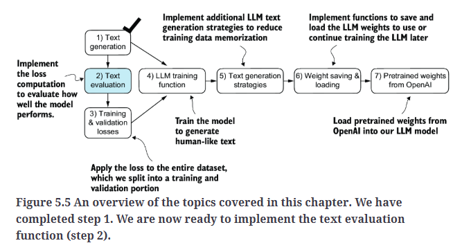
至此,文本生成部分结束,接下来是对文本生成质量的评估。
如Fig5.6所示,我们需要让正确单词的概率越高越好。
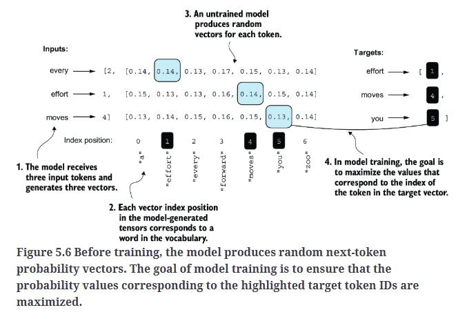
我们可以使用如下代码打印与目标token对应的初始softmax概率分数:
1
2
3
4
5
6
7
text_idx = 0
target_probas_1 = probas[text_idx, [0, 1, 2], targets[text_idx]]
print("Text 1:", target_probas_1) #Text 1: tensor([7.4540e-05, 3.1061e-05, 1.1563e-05])

text_idx = 1
target_probas_2 = probas[text_idx, [0, 1, 2], targets[text_idx]]
print("Text 2:", target_probas_2) #Text 2: tensor([1.0337e-05, 5.6776e-05, 4.7559e-06])
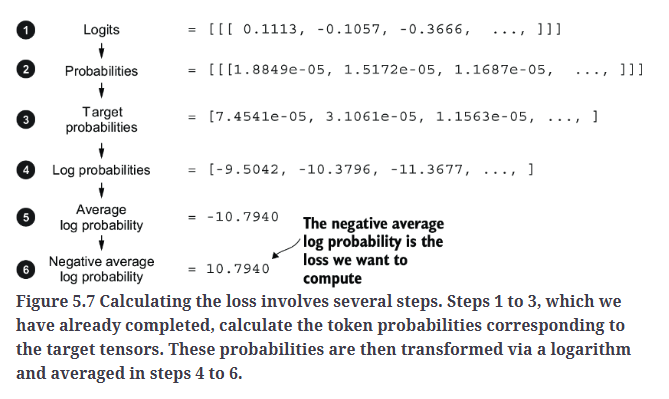
接下来,我们计算target_probas_1和target_probas_2的损失,主要步骤如Fig5.7所示。
1
2
3
4
5
6
7
8
9
10
# Compute logarithm of all token probabilities
log_probas = torch.log(torch.cat((target_probas_1, target_probas_2)))
print(log_probas) #tensor([ -9.5042, -10.3796, -11.3677, -11.4798,  -9.7764, -12.2561])

# Calculate the average probability for each token
avg_log_probas = torch.mean(log_probas)
print(avg_log_probas) #tensor(-10.7940)

neg_avg_log_probas = avg_log_probas * -1
print(neg_avg_log_probas) #tensor(10.7940)
loss部分可参考:交叉熵损失函数。
上述代码可以简化,直接调用PyTorch的cross_entropy接口:
1
2
3
4
5
6
7
8
9
10
11
12
13
14
# Logits have shape (batch_size, num_tokens, vocab_size)
print("Logits shape:", logits.shape) #Logits shape: torch.Size([2, 3, 50257])

# Targets have shape (batch_size, num_tokens)
print("Targets shape:", targets.shape) #Targets shape: torch.Size([2, 3])

logits_flat = logits.flatten(0, 1)
targets_flat = targets.flatten()

print("Flattened logits:", logits_flat.shape) #Flattened logits: torch.Size([6, 50257])
print("Flattened targets:", targets_flat.shape) #Flattened targets: torch.Size([6])

loss = torch.nn.functional.cross_entropy(logits_flat, targets_flat)
print(loss) #tensor(10.7940)
cross_entropy函数内部会自动执行softmax和对数似然计算。
perplexity是一种常与交叉熵损失一起使用的度量方法,常用于评估语言模型等任务的性能。它可以提供一种更直观的方式,帮助理解模型在预测序列下一个token时的不确定性。
perplexity衡量的是模型预测的概率分布和数据集中单词的实际分布的匹配程度。与损失类似,较低的perplexity表示模型的预测更接近实际分布,即模型的性能更好。
perplexity的计算方式为perplexity = torch.exp(loss),在上述代码示例中,perplexity的值为tensor(48725.8203)。
perplexity通常比原始损失值更易理解,因为它表示模型在每一步预测时的不确定性,相当于一个有效的词汇规模。在给定的示例中,这意味着模型在48725个词汇表token中不确定该生成哪个作为下一个token。
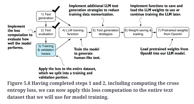
2.3.Calculating the training and validation set losses
我们首先需要准备训练集和验证集,用于训练LLM。然后,正如Fig5.8所示,我们将计算训练集和验证集的交叉熵损失。
在训练集和验证集上计算损失,为了演示方便,我们使用一个非常小的文本数据集:the-verdict.txt。
1
2
3
4
5
6
7
8
9
file_path = "the-verdict.txt"
with open(file_path, "r", encoding="utf-8") as file:
    text_data = file.read()

total_characters = len(text_data)
total_tokens = len(tokenizer.encode(text_data))

print("Characters:", total_characters) #Characters: 20479
print("Tokens:", total_tokens) #Tokens: 5145
接下来,我们划分训练集和验证集,在Fig5.9中为了演示方便,设max_length=6、batch size=2。
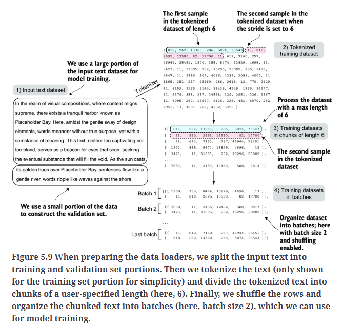
为了简化训练流程并提高效率,我们使用固定大小的文本块对模型进行训练。然而,在实际应用中,使用可变长度输入训练LLM可能更有益,因为这样可以提升模型的泛化能力,使其在不同类型的输入上表现更好。
90%的数据用于训练,剩余10%用于验证:
1
2
3
4
5
6
7
8
9
10
11
12
13
14
15
16
17
18
19
20
21
22
23
24
25
26
27
28
29
30
from previous_chapters import create_dataloader_v1

# Train/validation ratio
train_ratio = 0.90
split_idx = int(train_ratio * len(text_data))
train_data = text_data[:split_idx]
val_data = text_data[split_idx:]


torch.manual_seed(123)

train_loader = create_dataloader_v1(
    train_data,
    batch_size=2,
    max_length=GPT_CONFIG_124M["context_length"],
    stride=GPT_CONFIG_124M["context_length"],
    drop_last=True,
    shuffle=True,
    num_workers=0
)

val_loader = create_dataloader_v1(
    val_data,
    batch_size=2,
    max_length=GPT_CONFIG_124M["context_length"],
    stride=GPT_CONFIG_124M["context_length"],
    drop_last=False,
    shuffle=False,
    num_workers=0
)
我们使用了相对较小的batch size,以减少计算资源的需求。在实际应用中,训练LLM时,batch size可能会达到1024或更大。
1
2
3
4
5
6
7
print("Train loader:")
for x, y in train_loader:
    print(x.shape, y.shape)

print("\nValidation loader:")
for x, y in val_loader:
    print(x.shape, y.shape)
输出为:
1
2
3
4
5
6
7
8
9
10
11
12
13
Train loader:
torch.Size([2, 256]) torch.Size([2, 256])
torch.Size([2, 256]) torch.Size([2, 256])
torch.Size([2, 256]) torch.Size([2, 256])
torch.Size([2, 256]) torch.Size([2, 256])
torch.Size([2, 256]) torch.Size([2, 256])
torch.Size([2, 256]) torch.Size([2, 256])
torch.Size([2, 256]) torch.Size([2, 256])
torch.Size([2, 256]) torch.Size([2, 256])
torch.Size([2, 256]) torch.Size([2, 256])

Validation loader:
torch.Size([2, 256]) torch.Size([2, 256])
1
2
3
4
5
6
7
8
9
10
11
train_tokens = 0
for input_batch, target_batch in train_loader:
    train_tokens += input_batch.numel()

val_tokens = 0
for input_batch, target_batch in val_loader:
    val_tokens += input_batch.numel()

print("Training tokens:", train_tokens) #Training tokens: 4608
print("Validation tokens:", val_tokens) #Validation tokens: 512
print("All tokens:", train_tokens + val_tokens) #All tokens: 5120
实现loss计算函数:
1
2
3
4
5
6
7
8
9
10
11
12
13
14
15
16
17
18
19
20
21
22
23
24
25
26
#计算单个batch的loss
def calc_loss_batch(input_batch, target_batch, model, device):
    # The transfer to a given device allows us to transfer the data to a GPU
    input_batch, target_batch = input_batch.to(device), target_batch.to(device)
    logits = model(input_batch)
    loss = torch.nn.functional.cross_entropy(logits.flatten(0, 1), target_batch.flatten())
    return loss

#计算所有batch的loss
def calc_loss_loader(data_loader, model, device, num_batches=None):
    total_loss = 0.
    if len(data_loader) == 0: #len(data_loader)返回batch的数量
        return float("nan")
    elif num_batches is None:
        num_batches = len(data_loader)
    else:
        # Reduce the number of batches to match the total number of batches in the data loader
        # if num_batches exceeds the number of batches in the data loader
        num_batches = min(num_batches, len(data_loader))
    for i, (input_batch, target_batch) in enumerate(data_loader):
        if i < num_batches:
            loss = calc_loss_batch(input_batch, target_batch, model, device)
            total_loss += loss.item()
        else:
            break
    return total_loss / num_batches
我们可以通过设置参数num_batches来指定只计算部分batch的损失。这在实际应用中非常有用,可以快速获得一个粗略的评估结果。
1
2
3
4
5
6
7
8
9
10
11
12
13
device = torch.device("cuda" if torch.cuda.is_available() else "cpu")

model.to(device) # no assignment model = model.to(device) necessary for nn.Module classes


torch.manual_seed(123) # For reproducibility due to the shuffling in the data loader

with torch.no_grad(): # Disable gradient tracking for efficiency because we are not training, yet
    train_loss = calc_loss_loader(train_loader, model, device)
    val_loss = calc_loss_loader(val_loader, model, device)

print("Training loss:", train_loss) #Training loss: 10.987583584255642
print("Validation loss:", val_loss) #Validation loss: 10.98110580444336
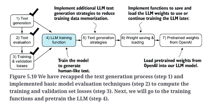
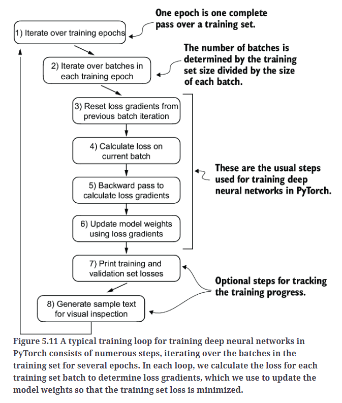
3.Training an LLM
如Fig5.11所示,我们会采用一个相对简单直接的训练循环,以使代码保持简洁且易于阅读。
1
2
3
4
5
6
7
8
9
10
11
12
13
14
15
16
17
18
19
20
21
22
23
24
25
26
27
28
29
30
31
32
33
34
35
36
37
38
39
40
41
42
43
44
45
46
47
48
49
50
51
52
53
54
55
56
57
58
59
60
61
62
63
64
65
66
67
68
69
def train_model_simple(model, train_loader, val_loader, optimizer, device, num_epochs,
                       eval_freq, eval_iter, start_context, tokenizer):
    # Initialize lists to track losses and tokens seen
    train_losses, val_losses, track_tokens_seen = [], [], []
    tokens_seen, global_step = 0, -1

    # Main training loop
    for epoch in range(num_epochs):
        model.train()  # Set model to training mode

        for input_batch, target_batch in train_loader:
            optimizer.zero_grad() # Reset loss gradients from previous batch iteration
            loss = calc_loss_batch(input_batch, target_batch, model, device)
            loss.backward() # Calculate loss gradients
            optimizer.step() # Update model weights using loss gradients
            tokens_seen += input_batch.numel()
            global_step += 1

            # Optional evaluation step
            if global_step % eval_freq == 0:
                train_loss, val_loss = evaluate_model(
                    model, train_loader, val_loader, device, eval_iter)
                train_losses.append(train_loss)
                val_losses.append(val_loss)
                track_tokens_seen.append(tokens_seen)
                print(f"Ep {epoch+1} (Step {global_step:06d}): "
                      f"Train loss {train_loss:.3f}, Val loss {val_loss:.3f}")

        # Print a sample text after each epoch
        generate_and_print_sample(
            model, tokenizer, device, start_context
        )

    return train_losses, val_losses, track_tokens_seen


def evaluate_model(model, train_loader, val_loader, device, eval_iter):
    model.eval()
    with torch.no_grad():
        train_loss = calc_loss_loader(train_loader, model, device, num_batches=eval_iter)
        val_loss = calc_loss_loader(val_loader, model, device, num_batches=eval_iter)
    model.train()
    return train_loss, val_loss


def generate_and_print_sample(model, tokenizer, device, start_context):
    model.eval()
    context_size = model.pos_emb.weight.shape[0]
    encoded = text_to_token_ids(start_context, tokenizer).to(device)
    with torch.no_grad():
        token_ids = generate_text_simple(
            model=model, idx=encoded,
            max_new_tokens=50, context_size=context_size
        )
    decoded_text = token_ids_to_text(token_ids, tokenizer)
    print(decoded_text.replace("\n", " "))  # Compact print format
    model.train()

torch.manual_seed(123)
model = GPTModel(GPT_CONFIG_124M)
model.to(device)
optimizer = torch.optim.AdamW(model.parameters(), lr=0.0004, weight_decay=0.1)

num_epochs = 10
train_losses, val_losses, tokens_seen = train_model_simple(
    model, train_loader, val_loader, optimizer, device,
    num_epochs=num_epochs, eval_freq=5, eval_iter=5,
    start_context="Every effort moves you", tokenizer=tokenizer
)
AdamW的讲解可见:【深度学习基础】第十九课:Adam优化算法。上述代码示例的输出为:
1
2
3
4
5
6
7
8
9
10
11
12
13
14
15
16
17
18
19
20
21
22
23
24
25
26
27
28
Ep 1 (Step 000000): Train loss 9.819, Val loss 9.926
Ep 1 (Step 000005): Train loss 8.070, Val loss 8.341
Every effort moves you,,,,,,,,,,,,.
Ep 2 (Step 000010): Train loss 6.624, Val loss 7.051
Ep 2 (Step 000015): Train loss 6.047, Val loss 6.599
Every effort moves you, and,, and,, and,,,, and,.
Ep 3 (Step 000020): Train loss 5.567, Val loss 6.483
Ep 3 (Step 000025): Train loss 5.507, Val loss 6.408
Every effort moves you, and, and of the of the of the, and, and. G. Gis, and, and, and, and, and, and, and, and, and, and, and, and, and, and, and,
Ep 4 (Step 000030): Train loss 5.090, Val loss 6.324
Ep 4 (Step 000035): Train loss 4.862, Val loss 6.334
Every effort moves you.  "I had been the picture-- the picture.               "I was a the of the of the of the of the of the picture"I had been the of
Ep 5 (Step 000040): Train loss 4.262, Val loss 6.217
Every effort moves you know the "I had been--I to me--as of the donkey.     "Oh, in the man of the picture--as Jack himself at the donkey--and it's the donkey--and it's it's
Ep 6 (Step 000045): Train loss 3.872, Val loss 6.151
Ep 6 (Step 000050): Train loss 3.334, Val loss 6.155
Every effort moves you know the "Oh, and.  "Oh, and in a little: "--I looked up, and in a little.       "Oh, and he was, and down the room, and I
Ep 7 (Step 000055): Train loss 3.329, Val loss 6.210
Ep 7 (Step 000060): Train loss 2.583, Val loss 6.143
Every effort moves you know the picture.  I glanced after him, and I was. I had been his pictures's an the fact, and I felt. I was his pictures--I had not the picture. I was, and down the room, I was
Ep 8 (Step 000065): Train loss 2.089, Val loss 6.168
Ep 8 (Step 000070): Train loss 1.759, Val loss 6.241
Every effort moves you?"  "Yes--I glanced after him, and uncertain.  "I looked up, with the fact, the cigars you like."  He placed them at my elbow and as he said, and down the room, when I
Ep 9 (Step 000075): Train loss 1.394, Val loss 6.229
Ep 9 (Step 000080): Train loss 1.074, Val loss 6.274
Every effort moves you know," was one of the picture for nothing--I told Mrs.  "Once, I was, in fact, and to see a smile behind his close grayish beard--as if he had the donkey. "There were days when I
Ep 10 (Step 000085): Train loss 0.806, Val loss 6.364
Every effort moves you?"  "Yes--quite insensible to the irony. She wanted him vindicated--and by me!"  He laughed again, and threw back his head to look up at the sketch of the donkey. "There were days when I
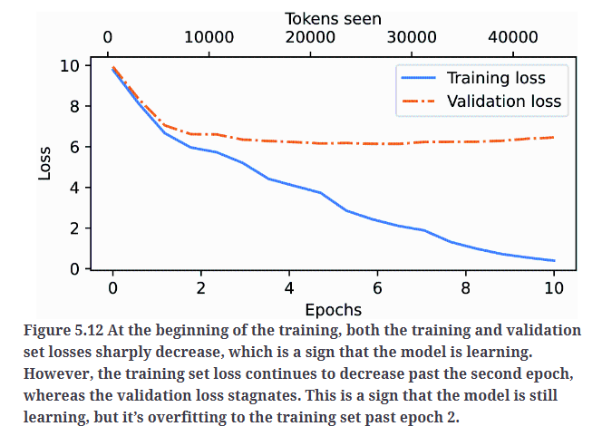
从上述训练过程可以看出,随着训练集loss的下降,文本生成质量逐步从随机无序的符号转变为有意义、符合语法的文本。相比训练集loss,验证集loss并没有下降到很低的值,这种情况表明模型可能存在一定程度的过拟合。在实践中,通常的解决办法是使用更大的数据集来训练模型。
1
2
3
4
5
6
7
8
9
10
11
12
13
14
15
16
17
18
19
20
21
22
23
24
25
26
import matplotlib.pyplot as plt
from matplotlib.ticker import MaxNLocator


def plot_losses(epochs_seen, tokens_seen, train_losses, val_losses):
    fig, ax1 = plt.subplots(figsize=(5, 3))

    # Plot training and validation loss against epochs
    ax1.plot(epochs_seen, train_losses, label="Training loss")
    ax1.plot(epochs_seen, val_losses, linestyle="-.", label="Validation loss")
    ax1.set_xlabel("Epochs")
    ax1.set_ylabel("Loss")
    ax1.legend(loc="upper right")
    ax1.xaxis.set_major_locator(MaxNLocator(integer=True))  # only show integer labels on x-axis

    # Create a second x-axis for tokens seen
    ax2 = ax1.twiny()  # Create a second x-axis that shares the same y-axis
    ax2.plot(tokens_seen, train_losses, alpha=0)  # Invisible plot for aligning ticks
    ax2.set_xlabel("Tokens seen")

    fig.tight_layout()  # Adjust layout to make room
    plt.savefig("loss-plot.pdf")
    plt.show()

epochs_tensor = torch.linspace(0, num_epochs, len(train_losses))
plot_losses(epochs_tensor, tokens_seen, train_losses, val_losses)
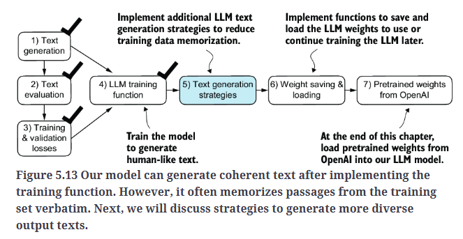
4.Decoding strategies to control randomness
在本部分,我们将关注文本生成策略,也称为解码策略,以使生成的文本更自然、更具原创性。首先,我们会简要回顾下之前实现的基础函数generate_text_simple。然后,我们将介绍两种高级的文本生成策略:temperature scaling和top-k sampling,以改善文本生成质量。
我们首先需要将模型从GPU转移回CPU,因为对于这种推理任务而言,使用较小的模型并在CPU上运行就已经足够,不再需要GPU。此外,在训练完成后,将模型设置为评估模式,以关闭像dropout等层的随机特性,确保推理时的结果稳定。
1
2
3
4
5
6
7
8
9
10
11
12
13
model.to("cpu")
model.eval()

tokenizer = tiktoken.get_encoding("gpt2")

token_ids = generate_text_simple(
    model=model,
    idx=text_to_token_ids("Every effort moves you", tokenizer),
    max_new_tokens=25,
    context_size=GPT_CONFIG_124M["context_length"]
)

print("Output text:\n", token_ids_to_text(token_ids, tokenizer))
输出为:
1
2
3
4
Output text:
 Every effort moves you?"

"Yes--quite insensible to the irony. She wanted him vindicated--and by me!"
如前所述,在每一步的文本生成过程中,模型都会从词汇表中选择概率得分最高的token作为生成的下一个token。这意味着,即使我们多次运行之前的generate_text_simple函数并使用相同的输入文本,LLM生成的输出文本也将始终保持不变。
4.1.Temperature scaling
temperature scaling在生成下一个token时引入了概率选择。在之前的generate_text_simple函数中,我们总是选择概率最大的token作为下一个token,这种策略被称为贪心解码(greedy decoding)。而为了生成更加多样化的文本,我们可以不使用argmax,而改为从概率分布中进行采样。
为了通过一个具体的例子来说明这种概率采样过程,我们将用一个非常小的词汇表,简单地展示一下生成下一个token的具体过程:
1
2
3
4
5
6
7
8
9
10
11
12
13
14
15
16
17
18
19
20
21
22
23
24
25
vocab = {
    "closer": 0,
    "every": 1,
    "effort": 2,
    "forward": 3,
    "inches": 4,
    "moves": 5,
    "pizza": 6,
    "toward": 7,
    "you": 8,
}

inverse_vocab = {v: k for k, v in vocab.items()}

# Suppose input is "every effort moves you", and the LLM
# returns the following logits for the next token:
next_token_logits = torch.tensor(
    [4.51, 0.89, -1.90, 6.75, 1.63, -1.62, -1.89, 6.28, 1.79]
)

probas = torch.softmax(next_token_logits, dim=0)
next_token_id = torch.argmax(probas).item()

# The next generated token is then as follows:
print(inverse_vocab[next_token_id]) #forward
为了实现概率采样过程,我们现在可以用PyTorch中的multinomial函数替换之前的argmax函数:
1
2
3
torch.manual_seed(123)
next_token_id = torch.multinomial(probas, num_samples=1).item()
print(inverse_vocab[next_token_id]) #forward
输出仍然是"forward",和之前一样,为什么会这样呢?因为multinomial函数是根据每个token的概率得分进行抽样的。因为"forward"是概率最大的token,因此绝大部分情况下,multinomial会选择它,但并非每次都会选中。为了更清晰地说明这一点,我们可以实现一个函数,将这个采样过程重复1000次:
1
2
3
4
5
6
7
8
def print_sampled_tokens(probas):
    torch.manual_seed(123) # Manual seed for reproducibility
    sample = [torch.multinomial(probas, num_samples=1).item() for i in range(1_000)]
    sampled_ids = torch.bincount(torch.tensor(sample))
    for i, freq in enumerate(sampled_ids):
        print(f"{freq} x {inverse_vocab[i]}")

print_sampled_tokens(probas)
输出为:
1
2
3
4
5
6
7
8
9
71 x closer
2 x every
0 x effort
544 x forward
2 x inches
1 x moves
0 x pizza
376 x toward
4 x you
我们还可以通过temperature scaling进一步控制概率分布及选择过程。temperature scaling实际上就是将logits除以一个大于0的数字:
1
2
3
4
5
6
7
8
9
def softmax_with_temperature(logits, temperature):
    scaled_logits = logits / temperature
    return torch.softmax(scaled_logits, dim=0)

# Temperature values
temperatures = [1, 0.1, 5]  # Original, higher confidence, and lower confidence

# Calculate scaled probabilities
scaled_probas = [softmax_with_temperature(next_token_logits, T) for T in temperatures]
当temperature大于1时,token的概率分布会变得更加均匀;而当temperature小于1时,概率分布则变得更加集中。我们可以通过绘制原始概率与使用不同temperature值后的概率的对比图,来直观地说明这一点:
1
2
3
4
5
6
7
8
9
10
11
12
13
14
15
16
# Plotting
x = torch.arange(len(vocab))
bar_width = 0.15

fig, ax = plt.subplots(figsize=(5, 3))
for i, T in enumerate(temperatures):
    rects = ax.bar(x + i * bar_width, scaled_probas[i], bar_width, label=f'Temperature = {T}')

ax.set_ylabel('Probability')
ax.set_xticks(x)
ax.set_xticklabels(vocab.keys(), rotation=90)
ax.legend()

plt.tight_layout()
plt.savefig("temperature-plot.pdf")
plt.show()
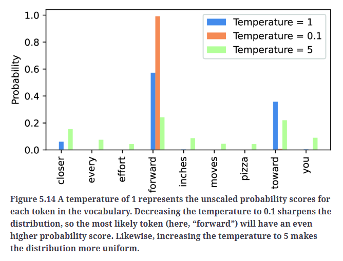
temperature越高,生成文本的多样性就越高,也越可能生成一些无意义的文本。
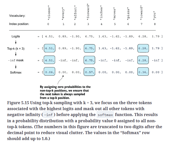
4.2.Top-k sampling
使用top-k sampling来进一步改善文本生成的结果。在top-k sampling中,我们将候选token限制为前k个最可能的token,并屏蔽其他token,如Fig5.15所示。
1
2
3
4
5
6
7
8
9
10
11
12
13
14
15
16
top_k = 3
top_logits, top_pos = torch.topk(next_token_logits, top_k)

print("Top logits:", top_logits) #Top logits: tensor([6.7500, 6.2800, 4.5100])
print("Top positions:", top_pos) #Top positions: tensor([3, 7, 0])

new_logits = torch.where(
    condition=next_token_logits < top_logits[-1], #Identifies logits less than the minimum in the top 3
    input=torch.tensor(float("-inf")), #Assigns –inf to these lower logits
    other=next_token_logits #Retains the original logits for all other tokens
)

print(new_logits) #tensor([4.5100,   -inf,   -inf, 6.7500,   -inf,   -inf,   -inf, 6.2800,   -inf])

topk_probas = torch.softmax(new_logits, dim=0)
print(topk_probas) #tensor([0.0615, 0.0000, 0.0000, 0.5775, 0.0000, 0.0000, 0.0000, 0.3610, 0.0000])
4.3.Modifying the text generation function
现在,让我们结合temperature scaling和top-k sampling,对之前用于生成文本的generate_text_simple函数进行修改,并创建一个新的generate函数。
1
2
3
4
5
6
7
8
9
10
11
12
13
14
15
16
17
18
19
20
21
22
23
24
25
26
27
28
29
30
31
32
33
34
35
36
37
38
39
40
41
42
43
44
45
46
47
48
49
50
def generate(model, idx, max_new_tokens, context_size, temperature=0.0, top_k=None, eos_id=None):

    # For-loop is the same as before: Get logits, and only focus on last time step
    for _ in range(max_new_tokens):
        idx_cond = idx[:, -context_size:]
        with torch.no_grad():
            logits = model(idx_cond)
        logits = logits[:, -1, :]

        # New: Filter logits with top_k sampling
        if top_k is not None:
            # Keep only top_k values
            top_logits, _ = torch.topk(logits, top_k)
            min_val = top_logits[:, -1]
            logits = torch.where(logits < min_val, torch.tensor(float("-inf")).to(logits.device), logits)

        # New: Apply temperature scaling
        if temperature > 0.0:
            logits = logits / temperature

            # Apply softmax to get probabilities
            probs = torch.softmax(logits, dim=-1)  # (batch_size, context_len)

            # Sample from the distribution
            idx_next = torch.multinomial(probs, num_samples=1)  # (batch_size, 1)

        # Otherwise same as before: get idx of the vocab entry with the highest logits value
        else:
            idx_next = torch.argmax(logits, dim=-1, keepdim=True)  # (batch_size, 1)

        if idx_next == eos_id:  # Stop generating early if end-of-sequence token is encountered and eos_id is specified
            break

        # Same as before: append sampled index to the running sequence
        idx = torch.cat((idx, idx_next), dim=1)  # (batch_size, num_tokens+1)

    return idx

torch.manual_seed(123)

token_ids = generate(
    model=model,
    idx=text_to_token_ids("Every effort moves you", tokenizer),
    max_new_tokens=15,
    context_size=GPT_CONFIG_124M["context_length"],
    top_k=25,
    temperature=1.4
)

print("Output text:\n", token_ids_to_text(token_ids, tokenizer))
输出为:
1
2
Output text:
 Every effort moves you know began to happen a little wild--I was such a good; and
5.Loading and saving model weights in PyTorch

1
2
#save
torch.save(model.state_dict(), "model.pth")
推荐的方法是保存模型的state_dict,其会返回一个包含模型所有参数的字典。.pth扩展名是PyTorch文件的惯例,但实际上,我们可以使用任何文件扩展名。
1
2
3
4
5
#load
model = GPTModel(GPT_CONFIG_124M)
device = torch.device("cuda" if torch.cuda.is_available() else "cpu")
model.load_state_dict(torch.load("model.pth", map_location=device, weights_only=True))
model.eval();
如果我们计划在之后继续对模型进行预训练,例如使用第3部分定义的train_model_simple函数,那么建议同时保存优化器的状态,以便在后续训练时恢复优化器的参数。
自适应优化器(如AdamW)会为每个模型权重存储额外的参数。AdamW通过历史数据动态调整每个模型参数的学习率。如果不保存优化器状态,优化器将在下次训练时重新初始化,这可能会导致模型学习效果不佳,甚至无法正确收敛,从而丧失生成连贯文本的能力。使用torch.save,我们可以同时保存模型和优化器的state_dict,如下所示:
1
2
3
4
5
6
7
8
9
10
11
12
13
14
15
16
17
#save
torch.save({
    "model_state_dict": model.state_dict(),
    "optimizer_state_dict": optimizer.state_dict(),
    },
    "model_and_optimizer.pth"
)

#load
checkpoint = torch.load("model_and_optimizer.pth", weights_only=True)

model = GPTModel(GPT_CONFIG_124M)
model.load_state_dict(checkpoint["model_state_dict"])

optimizer = torch.optim.AdamW(model.parameters(), lr=0.0005, weight_decay=0.1)
optimizer.load_state_dict(checkpoint["optimizer_state_dict"])
model.train();
6.Loading pretrained weights from OpenAI
OpenAI公开提供了GPT-2模型的权重。需要注意的是,OpenAI最初是使用TensorFlow保存GPT-2的权重。
1
2
3
4
5
6
#需要先确保安装了tensorflow和tqdm

# Relative import from the gpt_download.py contained in this folder
from gpt_download import download_and_load_gpt2 #作者把模型下载的代码封装到了gpt_download中

settings, params = download_and_load_gpt2(model_size="124M", models_dir="gpt2")
下载过程:
1
2
3
4
5
6
7
checkpoint: 100%|██████████| 77.0/77.0 [00:00<00:00, 38.5kiB/s]
encoder.json: 100%|██████████| 1.04M/1.04M [00:02<00:00, 466kiB/s]
hparams.json: 100%|██████████| 90.0/90.0 [00:00<00:00, 89.7kiB/s]
model.ckpt.data-00000-of-00001: 100%|██████████| 498M/498M [01:28<00:00, 5.61MiB/s]
model.ckpt.index: 100%|██████████| 5.21k/5.21k [00:00<00:00, 3.06MiB/s]
model.ckpt.meta: 100%|██████████| 471k/471k [00:01<00:00, 347kiB/s]
vocab.bpe: 100%|██████████| 456k/456k [00:01<00:00, 332kiB/s]
1
2
print("Settings:", settings) #Settings: {'n_vocab': 50257, 'n_ctx': 1024, 'n_embd': 768, 'n_head': 12, 'n_layer': 12}
print("Parameter dictionary keys:", params.keys()) #Parameter dictionary keys: dict_keys(['blocks', 'b', 'g', 'wpe', 'wte'])
settings和params都是Python字典。settings保存的是LLM的架构设置,类似于我们之前定义的GPT_CONFIG_124M。params保存实际的权重张量。
1
2
3
#查看嵌入层的权重
print(params["wte"])
print("Token embedding weight tensor dimensions:", params["wte"].shape)
输出为:
1
2
3
4
5
6
7
8
9
10
11
12
13
14
[[-0.11010301 -0.03926672  0.03310751 ... -0.1363697   0.01506208
   0.04531523]
 [ 0.04034033 -0.04861503  0.04624869 ...  0.08605453  0.00253983
   0.04318958]
 [-0.12746179  0.04793796  0.18410145 ...  0.08991534 -0.12972379
  -0.08785918]
 ...
 [-0.04453601 -0.05483596  0.01225674 ...  0.10435229  0.09783269
  -0.06952604]
 [ 0.1860082   0.01665728  0.04611587 ... -0.09625227  0.07847701
  -0.02245961]
 [ 0.05135201 -0.02768905  0.0499369  ...  0.00704835  0.15519823
   0.12067825]]
Token embedding weight tensor dimensions: (50257, 768)
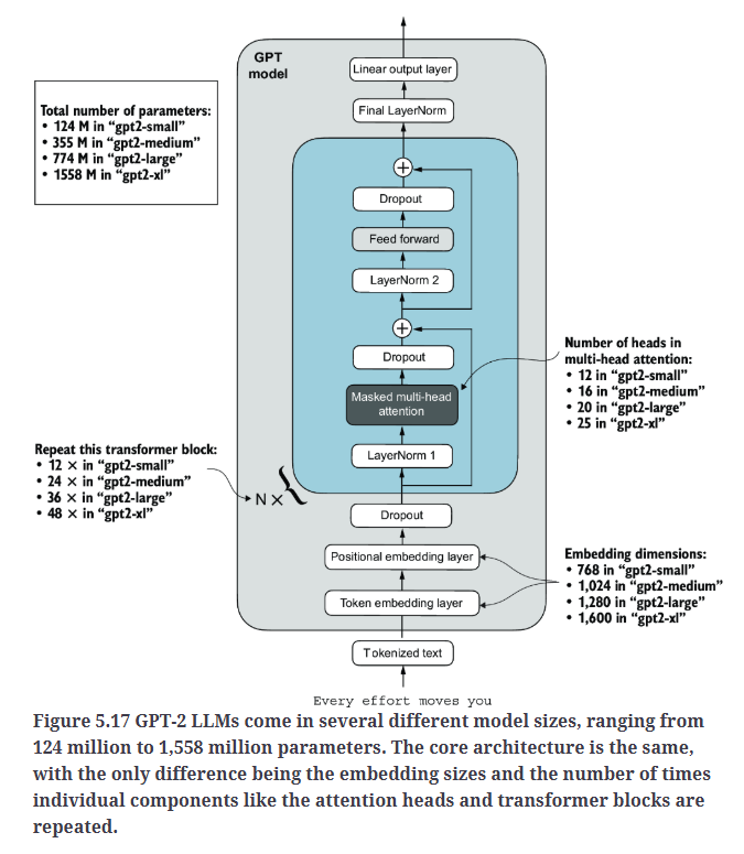
我们下载并加载了最小的GPT-2模型的权重。此外,OpenAI还提供了更大规模的模型权重,包括355M、774M和1558M。这些不同规模的GPT模型整体架构相同,区别如Fig5.17所示。
在将GPT-2模型权重加载到Python后,我们仍然需要将这些权重从settings和params转移到GPTModel实例中。首先,我们创建一个字典,用于列出不同规模的GPT模型之间的区别:
1
2
3
4
5
6
7
8
9
10
11
12
13
14
15
16
# Define model configurations in a dictionary for compactness
model_configs = {
    "gpt2-small (124M)": {"emb_dim": 768, "n_layers": 12, "n_heads": 12},
    "gpt2-medium (355M)": {"emb_dim": 1024, "n_layers": 24, "n_heads": 16},
    "gpt2-large (774M)": {"emb_dim": 1280, "n_layers": 36, "n_heads": 20},
    "gpt2-xl (1558M)": {"emb_dim": 1600, "n_layers": 48, "n_heads": 25},
}

# Copy the base configuration and update with specific model settings
model_name = "gpt2-small (124M)"  # Example model name
NEW_CONFIG = GPT_CONFIG_124M.copy()
NEW_CONFIG.update(model_configs[model_name])
NEW_CONFIG.update({"context_length": 1024, "qkv_bias": True})

gpt = GPTModel(NEW_CONFIG)
gpt.eval();
默认情况下,GPTModel实例在初始化时会使用随机权重进行预训练。要使用OpenAI提供的模型权重,最后一步是用params中加载的权重覆盖这些随机初始化的权重。为此,我们定义一个assign函数,用于检查两个张量或数组是否具有相同的维度或形状。
1
2
3
4
def assign(left, right):
    if left.shape != right.shape:
        raise ValueError(f"Shape mismatch. Left: {left.shape}, Right: {right.shape}")
    return torch.nn.Parameter(torch.tensor(right))
接下来,我们定义一个load_weights_into_gpt函数,该函数将params中的权重加载到GPTModel实例gpt中。
1
2
3
4
5
6
7
8
9
10
11
12
13
14
15
16
17
18
19
20
21
22
23
24
25
26
27
28
29
30
31
32
33
34
35
36
37
38
39
40
41
42
43
44
45
46
47
48
49
50
51
52
53
54
55
56
57
58
59
60
61
62
63
64
65
import numpy as np

def load_weights_into_gpt(gpt, params): #Sets the model’s positional and token embedding weights to those specified in params.
    gpt.pos_emb.weight = assign(gpt.pos_emb.weight, params['wpe'])
    gpt.tok_emb.weight = assign(gpt.tok_emb.weight, params['wte'])

    for b in range(len(params["blocks"])): #Iterates over each transformer block in the model
        q_w, k_w, v_w = np.split( #The np.split function is used to divide the attention and bias weights into three equal parts for the query, key, and value components.
            (params["blocks"][b]["attn"]["c_attn"])["w"], 3, axis=-1)
        gpt.trf_blocks[b].att.W_query.weight = assign(
            gpt.trf_blocks[b].att.W_query.weight, q_w.T)
        gpt.trf_blocks[b].att.W_key.weight = assign(
            gpt.trf_blocks[b].att.W_key.weight, k_w.T)
        gpt.trf_blocks[b].att.W_value.weight = assign(
            gpt.trf_blocks[b].att.W_value.weight, v_w.T)

        q_b, k_b, v_b = np.split(
            (params["blocks"][b]["attn"]["c_attn"])["b"], 3, axis=-1)
        gpt.trf_blocks[b].att.W_query.bias = assign(
            gpt.trf_blocks[b].att.W_query.bias, q_b)
        gpt.trf_blocks[b].att.W_key.bias = assign(
            gpt.trf_blocks[b].att.W_key.bias, k_b)
        gpt.trf_blocks[b].att.W_value.bias = assign(
            gpt.trf_blocks[b].att.W_value.bias, v_b)

        gpt.trf_blocks[b].att.out_proj.weight = assign(
            gpt.trf_blocks[b].att.out_proj.weight,
            params["blocks"][b]["attn"]["c_proj"]["w"].T)
        gpt.trf_blocks[b].att.out_proj.bias = assign(
            gpt.trf_blocks[b].att.out_proj.bias,
            params["blocks"][b]["attn"]["c_proj"]["b"])

        gpt.trf_blocks[b].ff.layers[0].weight = assign(
            gpt.trf_blocks[b].ff.layers[0].weight,
            params["blocks"][b]["mlp"]["c_fc"]["w"].T)
        gpt.trf_blocks[b].ff.layers[0].bias = assign(
            gpt.trf_blocks[b].ff.layers[0].bias,
            params["blocks"][b]["mlp"]["c_fc"]["b"])
        gpt.trf_blocks[b].ff.layers[2].weight = assign( #gpt.trf_blocks[b].ff.layers[1]是激活函数,所以跳过
            gpt.trf_blocks[b].ff.layers[2].weight,
            params["blocks"][b]["mlp"]["c_proj"]["w"].T)
        gpt.trf_blocks[b].ff.layers[2].bias = assign(
            gpt.trf_blocks[b].ff.layers[2].bias,
            params["blocks"][b]["mlp"]["c_proj"]["b"])

        gpt.trf_blocks[b].norm1.scale = assign(
            gpt.trf_blocks[b].norm1.scale,
            params["blocks"][b]["ln_1"]["g"])
        gpt.trf_blocks[b].norm1.shift = assign(
            gpt.trf_blocks[b].norm1.shift,
            params["blocks"][b]["ln_1"]["b"])
        gpt.trf_blocks[b].norm2.scale = assign(
            gpt.trf_blocks[b].norm2.scale,
            params["blocks"][b]["ln_2"]["g"])
        gpt.trf_blocks[b].norm2.shift = assign(
            gpt.trf_blocks[b].norm2.shift,
            params["blocks"][b]["ln_2"]["b"])

    gpt.final_norm.scale = assign(gpt.final_norm.scale, params["g"])
    gpt.final_norm.shift = assign(gpt.final_norm.shift, params["b"])
    gpt.out_head.weight = assign(gpt.out_head.weight, params["wte"]) #The original GPT-2 model by OpenAI reused the token embedding weights in the output layer to reduce the total number of parameters, which is a concept known as weight tying.


load_weights_into_gpt(gpt, params)
gpt.to(device);
现在我们可以调用之前实现的generate函数(见第4.3部分)来生成文本:
1
2
3
4
5
6
7
8
9
10
11
12
torch.manual_seed(123)

token_ids = generate(
    model=gpt,
    idx=text_to_token_ids("Every effort moves you", tokenizer).to(device),
    max_new_tokens=25,
    context_size=NEW_CONFIG["context_length"],
    top_k=50,
    temperature=1.5
)

print("Output text:\n", token_ids_to_text(token_ids, tokenizer))
输出为:
1
2
3
4
Output text:
 Every effort moves you as far as the hand can go until the end of your turn unless something happens

This would remove you from a battle