【从零开始构建大语言模型】系列博客为”Build a Large Language Model (From Scratch)”一书的个人读书笔记。
- 原书链接:Build a Large Language Model (From Scratch)。
- 官方示例代码:LLMs-from-scratch。
本文为原创文章,未经本人允许,禁止转载。转载请注明出处。
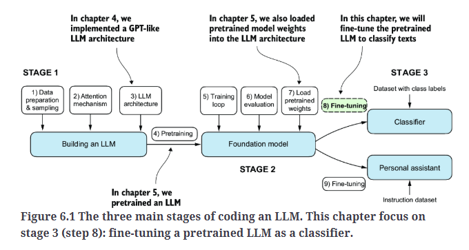
1.Fine-tuning for classification
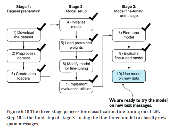
现在,我们对LLM进行fine-tune来完成特定的目标任务,比如文本分类。我们研究的具体示例是将短信分类为“垃圾短信”或“非垃圾短信”。
2.Different categories of fine-tuning
fine-tune语言模型最常见的方法是instruction fine-tuning和classification fine-tuning。Fig6.2展示了instruction fine-tuning的两种场景。
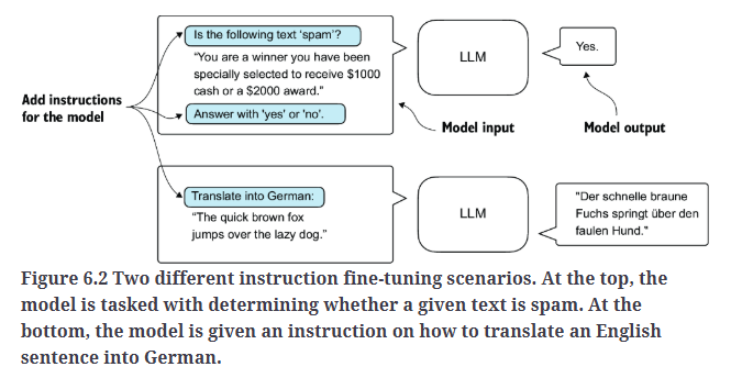
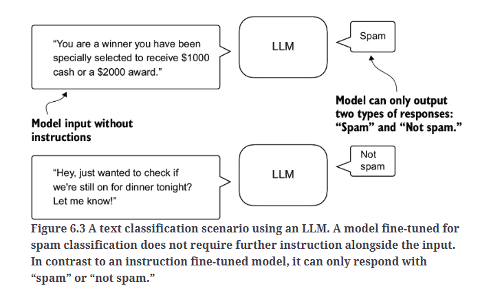
Fig6.3是一个classification fine-tuning的示例。
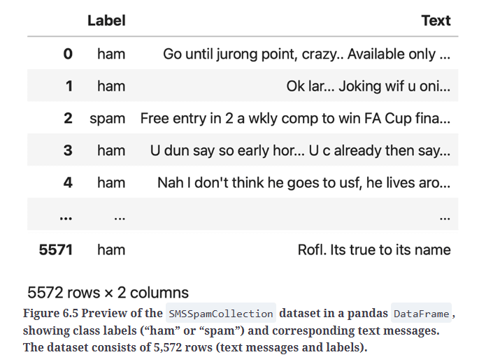
3.Preparing the dataset
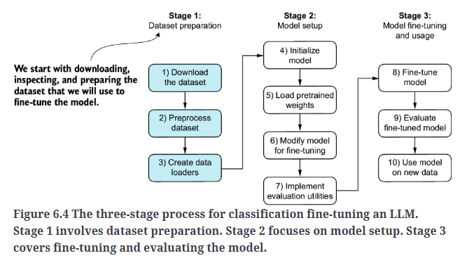
第一步,下载数据集。
1
2
3
4
5
6
7
8
9
10
11
12
13
14
15
16
17
18
19
20
21
22
23
24
25
26
27
28
29
30
31
32
33
34
35
36
#Downloading and unzipping the dataset
import urllib.request
import zipfile
import os
from pathlib import Path

url = "https://archive.ics.uci.edu/static/public/228/sms+spam+collection.zip"
zip_path = "sms_spam_collection.zip"
extracted_path = "sms_spam_collection"
data_file_path = Path(extracted_path) / "SMSSpamCollection.tsv"

def download_and_unzip_spam_data(url, zip_path, extracted_path, data_file_path):
    if data_file_path.exists():
        print(f"{data_file_path} already exists. Skipping download and extraction.")
        return

    # Downloading the file
    with urllib.request.urlopen(url) as response:
        with open(zip_path, "wb") as out_file:
            out_file.write(response.read())

    # Unzipping the file
    with zipfile.ZipFile(zip_path, "r") as zip_ref:
        zip_ref.extractall(extracted_path)

    # Add .tsv file extension
    original_file_path = Path(extracted_path) / "SMSSpamCollection"
    os.rename(original_file_path, data_file_path)
    print(f"File downloaded and saved as {data_file_path}")

download_and_unzip_spam_data(url, zip_path, extracted_path, data_file_path)

import pandas as pd

df = pd.read_csv(data_file_path, sep="\t", header=None, names=["Label", "Text"])
df
检查下类别标签的分布:
1
print(df["Label"].value_counts())
输出为:
1
2
3
4
Label
ham     4825
spam     747
Name: count, dtype: int64
为了简化处理,通过下采样使每个类别各包含747条样本。
1
2
3
4
5
6
7
8
9
10
11
12
13
14
15
16
17
#Creating a balanced dataset
def create_balanced_dataset(df):

    # Count the instances of "spam"
    num_spam = df[df["Label"] == "spam"].shape[0]

    # Randomly sample "ham" instances to match the number of "spam" instances
    ham_subset = df[df["Label"] == "ham"].sample(num_spam, random_state=123)

    # Combine ham "subset" with "spam"
    balanced_df = pd.concat([ham_subset, df[df["Label"] == "spam"]])

    return balanced_df


balanced_df = create_balanced_dataset(df)
print(balanced_df["Label"].value_counts())
输出为:
1
2
3
4
Label
ham     747
spam    747
Name: count, dtype: int64
将非垃圾短信(“ham”)标记为0,垃圾短信(“spam”)标记为1:
1
2
balanced_df["Label"] = balanced_df["Label"].map({"ham": 0, "spam": 1})
balanced_df
输出为:
1
2
3
4
5
6
7
8
9
10
11
12
13
	Label	Text
4307	0	Awww dat is sweet! We can think of something t...
4138	0	Just got to <#>
4831	0	The word "Checkmate" in chess comes from the P...
4461	0	This is wishing you a great day. Moji told me ...
5440	0	Thank you. do you generally date the brothas?
...	...	...
5537	1	Want explicit SEX in 30 secs? Ring 02073162414...
5540	1	ASKED 3MOBILE IF 0870 CHATLINES INCLU IN FREE ...
5547	1	Had your contract mobile 11 Mnths? Latest Moto...
5566	1	REMINDER FROM O2: To get 2.50 pounds free call...
5567	1	This is the 2nd time we have tried 2 contact u...
1494 rows × 2 columns
接下来,我们将数据集分成3部分:70%用于训练、10%用于验证、20%用于测试。
1
2
3
4
5
6
7
8
9
10
11
12
13
14
15
16
17
18
19
20
21
22
#Splitting the dataset
def random_split(df, train_frac, validation_frac):
    # Shuffle the entire DataFrame
    df = df.sample(frac=1, random_state=123).reset_index(drop=True)

    # Calculate split indices
    train_end = int(len(df) * train_frac)
    validation_end = train_end + int(len(df) * validation_frac)

    # Split the DataFrame
    train_df = df[:train_end]
    validation_df = df[train_end:validation_end]
    test_df = df[validation_end:]

    return train_df, validation_df, test_df

train_df, validation_df, test_df = random_split(balanced_df, 0.7, 0.1)
# Test size is implied to be 0.2 as the remainder

train_df.to_csv("train.csv", index=None)
validation_df.to_csv("validation.csv", index=None)
test_df.to_csv("test.csv", index=None)
4.Creating data loaders
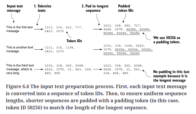
之前,我们使用滑动窗口生成统一长度的文本序列,但现在我们要处理的是一个包含不同文本长度的垃圾短信数据集,通常有两种解决办法:
- 将所有文本序列截断至数据集或batch中最短文本序列的长度。
- 将所有文本序列填充至数据集或batch中最长文本序列的长度。
第一种方式的计算成本较低,但可能会导致大量信息丢失,从而降低模型性能。因此,我们选择第二种方法。我们使用"<|endoftext|>"作为padding token,其对应的token ID为50256。
1
2
3
4
5
6
7
8
9
10
11
12
13
14
15
16
17
18
19
20
21
22
23
24
25
26
27
28
29
30
31
32
33
34
35
36
37
38
39
40
41
42
43
44
45
46
47
48
49
50
51
52
53
54
55
56
57
58
59
#Setting up a Pytorch Dataset class
import torch
from torch.utils.data import Dataset


class SpamDataset(Dataset):
    def __init__(self, csv_file, tokenizer, max_length=None, pad_token_id=50256):
        self.data = pd.read_csv(csv_file)

        # Pre-tokenize texts
        self.encoded_texts = [
            tokenizer.encode(text) for text in self.data["Text"]
        ]

        if max_length is None:
            self.max_length = self._longest_encoded_length()
        else:
            self.max_length = max_length
            # Truncate sequences if they are longer than max_length
            self.encoded_texts = [
                encoded_text[:self.max_length]
                for encoded_text in self.encoded_texts
            ]

        # Pad sequences to the longest sequence
        self.encoded_texts = [
            encoded_text + [pad_token_id] * (self.max_length - len(encoded_text))
            for encoded_text in self.encoded_texts
        ]

    def __getitem__(self, index):
        encoded = self.encoded_texts[index]
        label = self.data.iloc[index]["Label"]
        return (
            torch.tensor(encoded, dtype=torch.long),
            torch.tensor(label, dtype=torch.long)
        )

    def __len__(self):
        return len(self.data)

    def _longest_encoded_length(self):
        max_length = 0
        for encoded_text in self.encoded_texts:
            encoded_length = len(encoded_text)
            if encoded_length > max_length:
                max_length = encoded_length
        return max_length
        # Note: A more pythonic version to implement this method
        # is the following, which is also used in the next chapter:
        # return max(len(encoded_text) for encoded_text in self.encoded_texts)

train_dataset = SpamDataset(
    csv_file="train.csv",
    max_length=None,
    tokenizer=tokenizer
)

print(train_dataset.max_length) #120
如上述代码所示,最长文本序列的长度为120个token,并未超过我们所用模型的最大上下文长度(1024个token)。也就是说,我们最多可以将max_length设置为1024。
1
2
3
4
5
6
7
8
9
10
val_dataset = SpamDataset(
    csv_file="validation.csv",
    max_length=train_dataset.max_length, #保持和训练集一样的max_length
    tokenizer=tokenizer
)
test_dataset = SpamDataset(
    csv_file="test.csv",
    max_length=train_dataset.max_length, #保持和训练集一样的max_length
    tokenizer=tokenizer
)
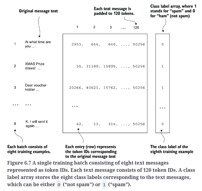
Fig6.7展示了batch size为8的情况。
1
2
3
4
5
6
7
8
9
10
11
12
13
14
15
16
17
18
19
20
21
22
23
24
25
26
27
28
29
30
31
32
33
34
35
36
37
#Creating PyTorch data loaders
from torch.utils.data import DataLoader

num_workers = 0 #This setting ensures compatibility with most computers.
batch_size = 8

torch.manual_seed(123)

train_loader = DataLoader(
    dataset=train_dataset,
    batch_size=batch_size,
    shuffle=True,
    num_workers=num_workers,
    drop_last=True,
)

val_loader = DataLoader(
    dataset=val_dataset,
    batch_size=batch_size,
    num_workers=num_workers,
    drop_last=False,
)

test_loader = DataLoader(
    dataset=test_dataset,
    batch_size=batch_size,
    num_workers=num_workers,
    drop_last=False,
)

print("Train loader:")
for input_batch, target_batch in train_loader:
    pass

#打印最后一个batch的张量维度
print("Input batch dimensions:", input_batch.shape)
print("Label batch dimensions", target_batch.shape)
输出为:
1
2
3
Train loader:
Input batch dimensions: torch.Size([8, 120])
Label batch dimensions torch.Size([8])
最后,为了了解数据集的规模,我们打印每个数据集中batch的数量。
1
2
3
print(f"{len(train_loader)} training batches") #130 training batches
print(f"{len(val_loader)} validation batches") #19 validation batches
print(f"{len(test_loader)} test batches") #38 test batches
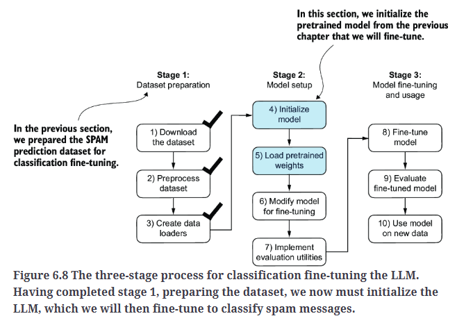
5.Initializing a model with pretrained weights
1
2
3
4
5
6
7
8
9
10
11
12
13
14
15
16
17
18
19
20
21
22
23
24
CHOOSE_MODEL = "gpt2-small (124M)"
INPUT_PROMPT = "Every effort moves"

BASE_CONFIG = {
    "vocab_size": 50257,     # Vocabulary size
    "context_length": 1024,  # Context length
    "drop_rate": 0.0,        # Dropout rate
    "qkv_bias": True         # Query-key-value bias
}

model_configs = {
    "gpt2-small (124M)": {"emb_dim": 768, "n_layers": 12, "n_heads": 12},
    "gpt2-medium (355M)": {"emb_dim": 1024, "n_layers": 24, "n_heads": 16},
    "gpt2-large (774M)": {"emb_dim": 1280, "n_layers": 36, "n_heads": 20},
    "gpt2-xl (1558M)": {"emb_dim": 1600, "n_layers": 48, "n_heads": 25},
}

BASE_CONFIG.update(model_configs[CHOOSE_MODEL])

assert train_dataset.max_length <= BASE_CONFIG["context_length"], (
    f"Dataset length {train_dataset.max_length} exceeds model's context "
    f"length {BASE_CONFIG['context_length']}. Reinitialize data sets with "
    f"`max_length={BASE_CONFIG['context_length']}`"
)
1
2
3
4
5
6
7
8
9
10
#Loading a pretrained GPT model
from gpt_download import download_and_load_gpt2
from previous_chapters import GPTModel, load_weights_into_gpt

model_size = CHOOSE_MODEL.split(" ")[-1].lstrip("(").rstrip(")")
settings, params = download_and_load_gpt2(model_size=model_size, models_dir="gpt2")

model = GPTModel(BASE_CONFIG)
load_weights_into_gpt(model, params)
model.eval();
GPTModel的定义见:Coding the GPT model,load_weights_into_gpt的定义见:Loading pretrained weights from OpenAI。
1
2
3
4
5
6
7
8
9
10
11
12
13
14
15
16
17
from previous_chapters import (
    generate_text_simple,
    text_to_token_ids,
    token_ids_to_text
)


text_1 = "Every effort moves you"

token_ids = generate_text_simple(
    model=model,
    idx=text_to_token_ids(text_1, tokenizer),
    max_new_tokens=15,
    context_size=BASE_CONFIG["context_length"]
)

print(token_ids_to_text(token_ids, tokenizer))
generate_text_simple的定义见:Generating text。
上述代码示例输出为:
1
2
3
Every effort moves you forward.

The first step is to understand the importance of your work
证明模型权重被正确加载。在将模型fine-tune为一个垃圾短信分类器之前,我们来看下其是否可以处理我们给出的instruction:
1
2
3
4
5
6
7
8
9
10
11
12
13
14
text_2 = (
    "Is the following text 'spam'? Answer with 'yes' or 'no':"
    " 'You are a winner you have been specially"
    " selected to receive $1000 cash or a $2000 award.'"
)

token_ids = generate_text_simple(
    model=model,
    idx=text_to_token_ids(text_2, tokenizer),
    max_new_tokens=23,
    context_size=BASE_CONFIG["context_length"]
)

print(token_ids_to_text(token_ids, tokenizer))
模型输出为:
1
2
3
Is the following text 'spam'? Answer with 'yes' or 'no': 'You are a winner you have been specially selected to receive $1000 cash or a $2000 award.'

The following text 'spam'? Answer with 'yes' or 'no': 'You are a winner
从输出结果来看,模型并不能遵照我们给出的instruction。这是因为它仅经过了预训练,并没有进行instruction fine-tuning。接下来我们对模型进行classification fine-tuning。
6.Adding a classification head
如Fig6.9所示,我们对输出层进行修改。
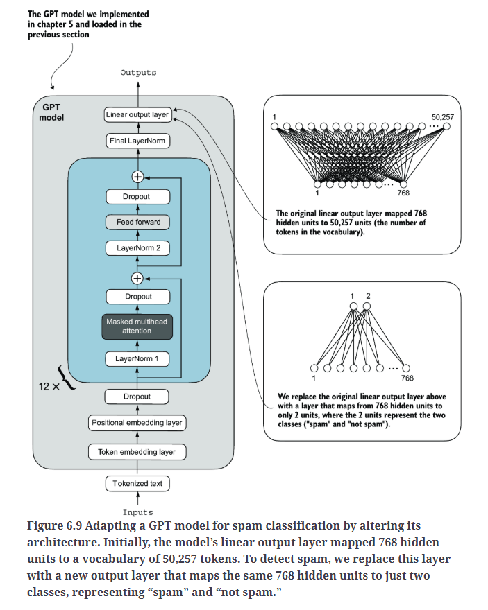
这是一个二分类问题,理论上我们可以使用单个输出节点,但这样做需要修改损失函数。因此,我们选择了一种更为通用的方法,即输出节点数量与类别数相匹配。
在我们开始修改之前,先来看下模型框架print(model):
1
2
3
4
5
6
7
8
9
10
11
12
13
14
15
16
17
18
19
20
21
22
23
24
25
26
27
28
29
30
GPTModel(
  (tok_emb): Embedding(50257, 768)
  (pos_emb): Embedding(1024, 768)
  (drop_emb): Dropout(p=0.0, inplace=False)
  (trf_blocks): Sequential(
    (0): TransformerBlock(
      (att): MultiHeadAttention(
        (W_query): Linear(in_features=768, out_features=768, bias=True)
        (W_key): Linear(in_features=768, out_features=768, bias=True)
        (W_value): Linear(in_features=768, out_features=768, bias=True)
        (out_proj): Linear(in_features=768, out_features=768, bias=True)
        (dropout): Dropout(p=0.0, inplace=False)
      )
      (ff): FeedForward(
        (layers): Sequential(
          (0): Linear(in_features=768, out_features=3072, bias=True)
          (1): GELU()
          (2): Linear(in_features=3072, out_features=768, bias=True)
        )
      )
      (norm1): LayerNorm()
      (norm2): LayerNorm()
      (drop_resid): Dropout(p=0.0, inplace=False)
    )
    (1): TransformerBlock(
...
  )
  (final_norm): LayerNorm()
  (out_head): Linear(in_features=768, out_features=50257, bias=False)
)
我们首先冻结模型,将所有层设置为不可训练:
1
2
for param in model.parameters():
    param.requires_grad = False
接着,替换输出层model.out_head:
1
2
3
4
5
#Adding a classification layer
torch.manual_seed(123)

num_classes = 2
model.out_head = torch.nn.Linear(in_features=BASE_CONFIG["emb_dim"], out_features=num_classes)
新的model.out_head输出层的requires_grad属性默认设置为True,这意味着它是模型中唯一会在训练过程中更新的层。从技术上讲,仅训练我们刚添加的输出层就足够了。然而,根据实验结果,发现微调额外的层可以显著提升模型的预测性能。因此,我们还将最后一个transformer block和最终的LayerNorm模块设置为可训练,如Fig6.10所示。

对应的代码:
1
2
3
4
5
for param in model.trf_blocks[-1].parameters():
    param.requires_grad = True

for param in model.final_norm.parameters():
    param.requires_grad = True
尽管我们添加了新的输出层,并将某些层标记为可训练或不可训练,但我们仍然可以像以前一样使用该模型。
1
2
3
4
5
6
7
8
9
10
inputs = tokenizer.encode("Do you have time")
inputs = torch.tensor(inputs).unsqueeze(0)
print("Inputs:", inputs)
print("Inputs dimensions:", inputs.shape) # shape: (batch_size, num_tokens)

with torch.no_grad():
    outputs = model(inputs)

print("Outputs:\n", outputs)
print("Outputs dimensions:", outputs.shape) # shape: (batch_size, num_tokens, num_classes)
输出为:
1
2
3
4
5
6
7
8
Inputs: tensor([[5211,  345,  423,  640]])
Inputs dimensions: torch.Size([1, 4])
Outputs:
 tensor([[[-1.5854,  0.9904],
         [-3.7235,  7.4548],
         [-2.2661,  6.6049],
         [-3.5983,  3.9902]]])
Outputs dimensions: torch.Size([1, 4, 2])
类似的输入以前会生成一个形状为[1, 4, 50257]的输出张量,其中50257代表词汇表大小。输出的行数对应于输入的token数量。然而,现在每个输出的维度是2而不是50257,这是因为我们替换了模型的输出层。
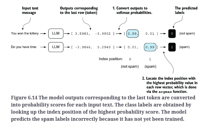
对于分类任务,我们将关注输出的最后一行,即对应于最后一个输出token的行,如Fig6.11所示。
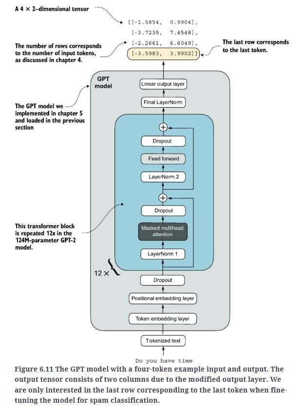
从输出张量中提取最后一个输出token:
1
print("Last output token:", outputs[:, -1, :]) #Last output token: tensor([[-3.5983,  3.9902]])
这里解释下我们为什么会特别关注最后一个输出token。因果注意力掩码使得每个token只能关注其当前位置及之前的token,确保每个token只能受到自己及其前面token的影响,如图6.12所示。
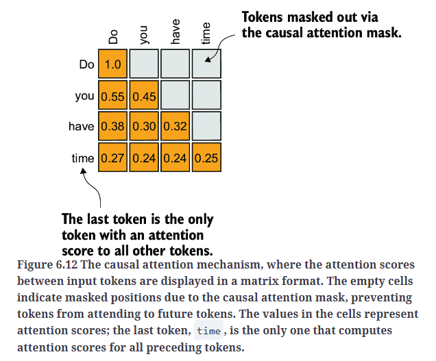
序列中的最后一个token累积了最多的信息,因为它是唯一能够访问所有前面token数据的token,因此,我们会专注于只处理最后一个token。
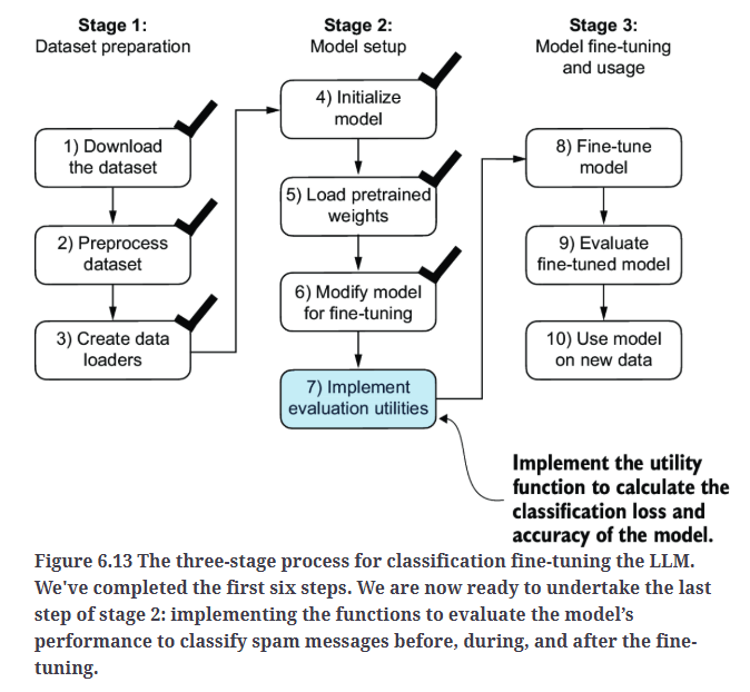
7.Calculating the classification loss and accuracy
1
2
3
4
print("Last output token:", outputs[:, -1, :]) #Last output token: tensor([[-3.5983,  3.9902]])
probas = torch.softmax(outputs[:, -1, :], dim=-1) #可省略
label = torch.argmax(probas)
print("Class label:", label.item()) #Class label: 1
定义一个计算分类正确率的函数:
1
2
3
4
5
6
7
8
9
10
11
12
13
14
15
16
17
18
19
20
21
22
#Calculating the classification accuracy
def calc_accuracy_loader(data_loader, model, device, num_batches=None):
    model.eval()
    correct_predictions, num_examples = 0, 0

    if num_batches is None:
        num_batches = len(data_loader)
    else:
        num_batches = min(num_batches, len(data_loader))
    for i, (input_batch, target_batch) in enumerate(data_loader):
        if i < num_batches:
            input_batch, target_batch = input_batch.to(device), target_batch.to(device)

            with torch.no_grad():
                logits = model(input_batch)[:, -1, :]  # Logits of last output token
            predicted_labels = torch.argmax(logits, dim=-1)

            num_examples += predicted_labels.shape[0]
            correct_predictions += (predicted_labels == target_batch).sum().item()
        else:
            break
    return correct_predictions / num_examples
让我们使用该函数在多个数据集上,计算10个batch的分类正确率:
1
2
3
4
5
6
7
8
9
10
11
12
13
14
15
16
17
18
19
20
21
22
23
24
25
26
27
device = torch.device("cuda" if torch.cuda.is_available() else "cpu")

# Note:
# Uncommenting the following lines will allow the code to run on Apple Silicon chips, if applicable,
# which is approximately 2x faster than on an Apple CPU (as measured on an M3 MacBook Air).
# As of this writing, in PyTorch 2.4, the results obtained via CPU and MPS were identical.
# However, in earlier versions of PyTorch, you may observe different results when using MPS.

#if torch.cuda.is_available():
#    device = torch.device("cuda")
#elif torch.backends.mps.is_available():
#    device = torch.device("mps")
#else:
#    device = torch.device("cpu")
#print(f"Running on {device} device.")

model.to(device) # no assignment model = model.to(device) necessary for nn.Module classes

torch.manual_seed(123) # For reproducibility due to the shuffling in the training data loader

train_accuracy = calc_accuracy_loader(train_loader, model, device, num_batches=10)
val_accuracy = calc_accuracy_loader(val_loader, model, device, num_batches=10)
test_accuracy = calc_accuracy_loader(test_loader, model, device, num_batches=10)

print(f"Training accuracy: {train_accuracy*100:.2f}%") #Training accuracy: 46.25%
print(f"Validation accuracy: {val_accuracy*100:.2f}%") #Validation accuracy: 45.00%
print(f"Test accuracy: {test_accuracy*100:.2f}%") #Test accuracy: 48.75%
正如我们所见,模型的预测准确率接近随机预测的水平,即50%左右。为了提升预测准确率,我们需要对模型进行fine-tune。
首先定义损失函数:
1
2
3
4
5
6
7
8
9
10
11
12
13
14
15
16
17
18
19
20
21
22
23
24
25
def calc_loss_batch(input_batch, target_batch, model, device):
    input_batch, target_batch = input_batch.to(device), target_batch.to(device)
    logits = model(input_batch)[:, -1, :]  # Logits of last output token
    loss = torch.nn.functional.cross_entropy(logits, target_batch)
    return loss

#Calculating the classification loss
# Same as in chapter 5
def calc_loss_loader(data_loader, model, device, num_batches=None):
    total_loss = 0.
    if len(data_loader) == 0:
        return float("nan")
    elif num_batches is None:
        num_batches = len(data_loader)
    else:
        # Reduce the number of batches to match the total number of batches in the data loader
        # if num_batches exceeds the number of batches in the data loader
        num_batches = min(num_batches, len(data_loader))
    for i, (input_batch, target_batch) in enumerate(data_loader):
        if i < num_batches:
            loss = calc_loss_batch(input_batch, target_batch, model, device)
            total_loss += loss.item()
        else:
            break
    return total_loss / num_batches
我们可以计算在每个数据集上的初始loss:
1
2
3
4
5
6
7
8
with torch.no_grad(): # Disable gradient tracking for efficiency because we are not training, yet
    train_loss = calc_loss_loader(train_loader, model, device, num_batches=5)
    val_loss = calc_loss_loader(val_loader, model, device, num_batches=5)
    test_loss = calc_loss_loader(test_loader, model, device, num_batches=5)

print(f"Training loss: {train_loss:.3f}") #Training loss: 2.453
print(f"Validation loss: {val_loss:.3f}") #Validation loss: 2.583
print(f"Test loss: {test_loss:.3f}") #Test loss: 2.322
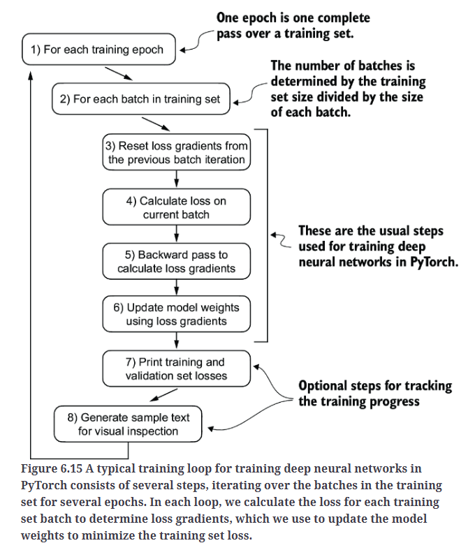
8.Fine-tuning the model on supervised data
fine-tune的训练流程基本和预训练是一样的,唯一的不同是我们计算的是分类精度而不是生成文本,如Fig6.15所示。
1
2
3
4
5
6
7
8
9
10
11
12
13
14
15
16
17
18
19
20
21
22
23
24
25
26
27
28
29
30
31
32
33
34
35
36
37
# Overall the same as `train_model_simple` in chapter 5
def train_classifier_simple(model, train_loader, val_loader, optimizer, device, num_epochs,
                            eval_freq, eval_iter):
    # Initialize lists to track losses and examples seen
    train_losses, val_losses, train_accs, val_accs = [], [], [], []
    examples_seen, global_step = 0, -1

    # Main training loop
    for epoch in range(num_epochs):
        model.train()  # Set model to training mode

        for input_batch, target_batch in train_loader:
            optimizer.zero_grad() # Reset loss gradients from previous batch iteration
            loss = calc_loss_batch(input_batch, target_batch, model, device)
            loss.backward() # Calculate loss gradients
            optimizer.step() # Update model weights using loss gradients
            examples_seen += input_batch.shape[0] # New: track examples instead of tokens
            global_step += 1

            # Optional evaluation step
            if global_step % eval_freq == 0:
                train_loss, val_loss = evaluate_model(
                    model, train_loader, val_loader, device, eval_iter)
                train_losses.append(train_loss)
                val_losses.append(val_loss)
                print(f"Ep {epoch+1} (Step {global_step:06d}): "
                      f"Train loss {train_loss:.3f}, Val loss {val_loss:.3f}")

        # Calculate accuracy after each epoch
        train_accuracy = calc_accuracy_loader(train_loader, model, device, num_batches=eval_iter)
        val_accuracy = calc_accuracy_loader(val_loader, model, device, num_batches=eval_iter)
        print(f"Training accuracy: {train_accuracy*100:.2f}% | ", end="")
        print(f"Validation accuracy: {val_accuracy*100:.2f}%")
        train_accs.append(train_accuracy)
        val_accs.append(val_accuracy)

    return train_losses, val_losses, train_accs, val_accs, examples_seen
calc_accuracy_loader的定义见第7部分,evaluate_model的定义见下:
1
2
3
4
5
6
7
8
# Same as chapter 5
def evaluate_model(model, train_loader, val_loader, device, eval_iter):
    model.eval()
    with torch.no_grad():
        train_loss = calc_loss_loader(train_loader, model, device, num_batches=eval_iter)
        val_loss = calc_loss_loader(val_loader, model, device, num_batches=eval_iter)
    model.train()
    return train_loss, val_loss
calc_loss_loader的定义见第7部分。接下来,我们初始化优化器,设置训练的epoch数量,并使用train_classifier_simple函数开始训练。在M3 MacBook Air上训练大约需要6分钟,而在V100或A100上训练则不到半分钟。
1
2
3
4
5
6
7
8
9
10
11
12
13
14
15
16
17
import time

start_time = time.time()

torch.manual_seed(123)

optimizer = torch.optim.AdamW(model.parameters(), lr=5e-5, weight_decay=0.1)

num_epochs = 5
train_losses, val_losses, train_accs, val_accs, examples_seen = train_classifier_simple(
    model, train_loader, val_loader, optimizer, device,
    num_epochs=num_epochs, eval_freq=50, eval_iter=5,
)

end_time = time.time()
execution_time_minutes = (end_time - start_time) / 60
print(f"Training completed in {execution_time_minutes:.2f} minutes.")
输出为:
1
2
3
4
5
6
7
8
9
10
11
12
13
14
15
16
17
18
19
Ep 1 (Step 000000): Train loss 2.153, Val loss 2.392
Ep 1 (Step 000050): Train loss 0.617, Val loss 0.637
Ep 1 (Step 000100): Train loss 0.523, Val loss 0.557
Training accuracy: 70.00% | Validation accuracy: 72.50%
Ep 2 (Step 000150): Train loss 0.561, Val loss 0.489
Ep 2 (Step 000200): Train loss 0.419, Val loss 0.397
Ep 2 (Step 000250): Train loss 0.409, Val loss 0.353
Training accuracy: 82.50% | Validation accuracy: 85.00%
Ep 3 (Step 000300): Train loss 0.333, Val loss 0.320
Ep 3 (Step 000350): Train loss 0.340, Val loss 0.306
Training accuracy: 90.00% | Validation accuracy: 90.00%
Ep 4 (Step 000400): Train loss 0.136, Val loss 0.200
Ep 4 (Step 000450): Train loss 0.153, Val loss 0.132
Ep 4 (Step 000500): Train loss 0.222, Val loss 0.137
Training accuracy: 100.00% | Validation accuracy: 97.50%
Ep 5 (Step 000550): Train loss 0.207, Val loss 0.143
Ep 5 (Step 000600): Train loss 0.083, Val loss 0.074
Training accuracy: 100.00% | Validation accuracy: 97.50%
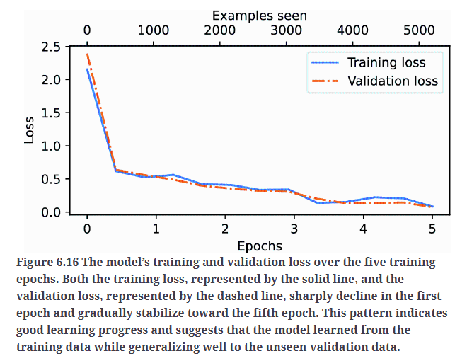
Training completed in 1.66 minutes.
使用Matplotlib绘制训练集和验证集的loss曲线:
1
2
3
4
5
6
7
8
9
10
11
12
13
14
15
16
17
18
19
20
21
22
23
24
25
26
#Plotting the classification loss
import matplotlib.pyplot as plt

def plot_values(epochs_seen, examples_seen, train_values, val_values, label="loss"):
    fig, ax1 = plt.subplots(figsize=(5, 3))

    # Plot training and validation loss against epochs
    ax1.plot(epochs_seen, train_values, label=f"Training {label}")
    ax1.plot(epochs_seen, val_values, linestyle="-.", label=f"Validation {label}")
    ax1.set_xlabel("Epochs")
    ax1.set_ylabel(label.capitalize())
    ax1.legend()

    # Create a second x-axis for examples seen
    ax2 = ax1.twiny()  # Create a second x-axis that shares the same y-axis
    ax2.plot(examples_seen, train_values, alpha=0)  # Invisible plot for aligning ticks
    ax2.set_xlabel("Examples seen")

    fig.tight_layout()  # Adjust layout to make room
    plt.savefig(f"{label}-plot.pdf")
    plt.show()

epochs_tensor = torch.linspace(0, num_epochs, len(train_losses))
examples_seen_tensor = torch.linspace(0, examples_seen, len(train_losses))

plot_values(epochs_tensor, examples_seen_tensor, train_losses, val_losses)
绘制准确率曲线:
1
2
3
4
epochs_tensor = torch.linspace(0, num_epochs, len(train_accs))
examples_seen_tensor = torch.linspace(0, examples_seen, len(train_accs))

plot_values(epochs_tensor, examples_seen_tensor, train_accs, val_accs, label="accuracy")
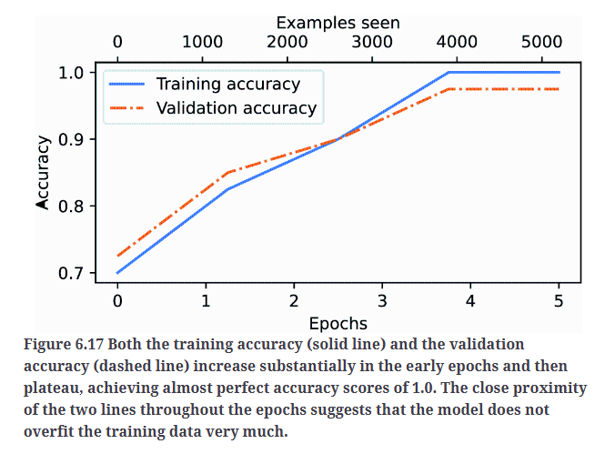
现在我们计算在训练集、验证集和测试集上的分类准确率:
1
2
3
4
5
6
7
train_accuracy = calc_accuracy_loader(train_loader, model, device)
val_accuracy = calc_accuracy_loader(val_loader, model, device)
test_accuracy = calc_accuracy_loader(test_loader, model, device)

print(f"Training accuracy: {train_accuracy*100:.2f}%") #Training accuracy: 97.21%
print(f"Validation accuracy: {val_accuracy*100:.2f}%") #Validation accuracy: 97.32%
print(f"Test accuracy: {test_accuracy*100:.2f}%") #Test accuracy: 95.67%
calc_accuracy_loader的定义见第7部分。上述结果可以看到,训练集和验证集的准确率要高于测试集,这可能是因为没有很好的泛化到测试集,这种情况很常见,可以通过调整模型设置来减少这种差距,例如增加dropout rate或调整优化器中的weight_decay参数。
9.Using the LLM as a spam classifier
1
2
3
4
5
6
7
8
9
10
11
12
13
14
15
16
17
18
19
20
21
22
23
24
25
26
27
28
29
30
31
32
33
34
35
36
37
38
39
40
41
42
#Using the model to classify new texts
def classify_review(text, model, tokenizer, device, max_length=None, pad_token_id=50256):
    model.eval()

    # Prepare inputs to the model
    input_ids = tokenizer.encode(text)
    supported_context_length = model.pos_emb.weight.shape[0]
    # Note: In the book, this was originally written as pos_emb.weight.shape[1] by mistake
    # It didn't break the code but would have caused unnecessary truncation (to 768 instead of 1024)

    # Truncate sequences if they too long
    input_ids = input_ids[:min(max_length, supported_context_length)]

    # Pad sequences to the longest sequence
    input_ids += [pad_token_id] * (max_length - len(input_ids))
    input_tensor = torch.tensor(input_ids, device=device).unsqueeze(0) # add batch dimension

    # Model inference
    with torch.no_grad():
        logits = model(input_tensor)[:, -1, :]  # Logits of the last output token
    predicted_label = torch.argmax(logits, dim=-1).item()

    # Return the classified result
    return "spam" if predicted_label == 1 else "not spam"

text_1 = (
    "You are a winner you have been specially"
    " selected to receive $1000 cash or a $2000 award."
)

print(classify_review(
    text_1, model, tokenizer, device, max_length=train_dataset.max_length
)) #spam

text_2 = (
    "Hey, just wanted to check if we're still on"
    " for dinner tonight? Let me know!"
)

print(classify_review(
    text_2, model, tokenizer, device, max_length=train_dataset.max_length
)) #not spam
最后,让我们保存模型,以便以后可以直接复用,而无需重新训练。我们可以使用torch.save方法来实现:
1
torch.save(model.state_dict(), "review_classifier.pth")
加载模型:
1
2
model_state_dict = torch.load("review_classifier.pth", map_location=device, weights_only=True)
model.load_state_dict(model_state_dict)