本文为原创文章，未经本人允许，禁止转载。转载请注明出处。

1.Introduction

github源码地址：https://github.com/WongKinYiu/yolov7。

本文提出的方法不仅在网络结构上进行优化，还将重点关注训练过程的优化。我们将引入一些优化模块和训练方法，虽然这些方法可能会增加训练成本，但不会提升推理成本，从而在不影响推理速度的前提下提高检测精度。我们将这些优化模块和训练方法称为trainable bag-of-freebies。

Fig1

2.Related work

不再赘述。

3.Architecture

3.1.Extended efficient layer aggregation networks

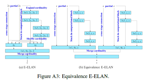
基于ELAN提出了Extended-ELAN（E-ELAN），如Fig2(d)所示。

Fig2

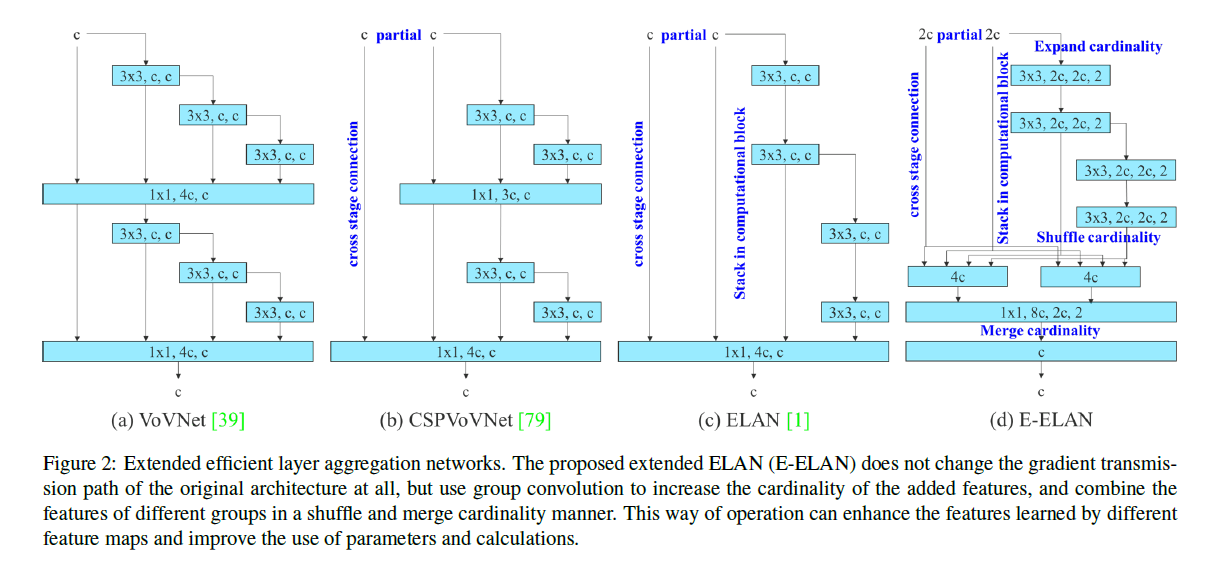
在Fig2(d)中，先解释几个概念，首先是cardinality，这个概念来自ResNeXt，表示分支路径的数量。Fig2(d)中的Expand cardinality是分组卷积的意思，”3x3, 2c, 2c, 2”表示使用$3 \times 3$卷积，输入通道数为2c，输出通道数也为2c，group数量为2。Shuffle cardinality就是channel shuffle操作。Fig2(d)详细展开如下所示：

但在实际代码实现时，作者使用了Fig2(d)的另一种等价结构，如下所示：

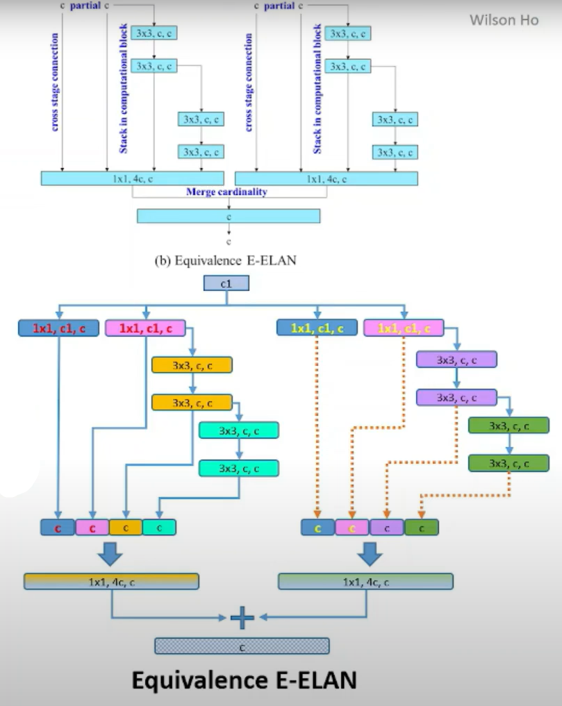
上下两张图是一个意思，其实就是并行了两个ELAN。

3.2.Model scaling for concatenation-based models

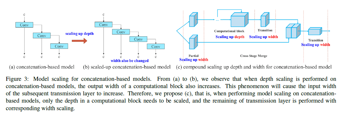
对于concatenation-based的架构，如Fig3(a)所示，如果我们想通过增加网络深度的方式来扩展网络模型，即Fig3(b)所示的形式，这样会导致concat之后的输出通道数变多，即不仅仅增加了深度，网络宽度也被迫增加，从而导致后续层的输入通道数增加，这会增加额外计算和参数，破坏了原有的比例关系。因此我们提出如Fig3(c)所示的方法，其核心思想就是通过transition layer来控制输出通道数。

4.Trainable bag-of-freebies

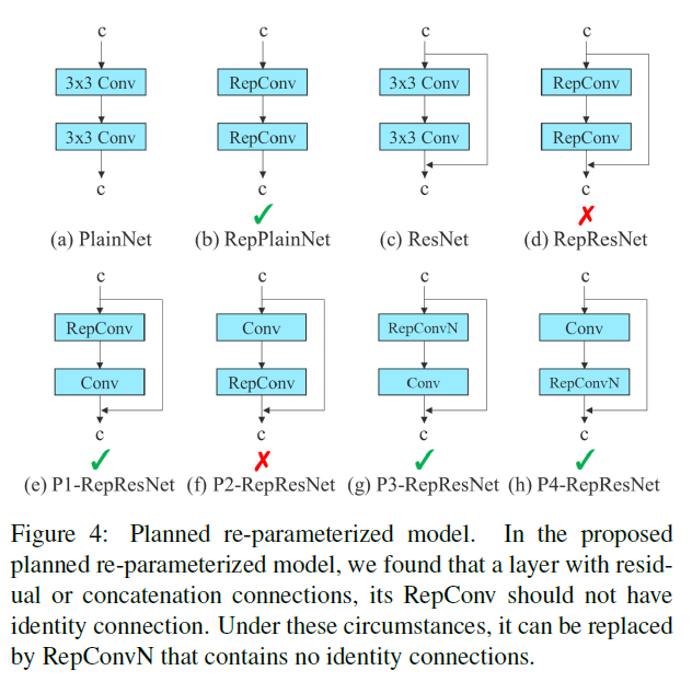
4.1.Planned re-parameterized convolution

当我们将RepConv直接应用于ResNet或DenseNet或其他框架时，模型精度会出现显著下降。因此我们重新设计了RepConv。

RepConv在一个卷积层中通常包含一个$3\times 3$卷积、一个$1\times 1$卷积和一个identity连接。我们发现identity连接破坏了ResNet的残差结构和DenseNet的concat操作，因此，我们去掉了RepConv中的identity连接，记为RepConvN。

4.2.Coarse for auxiliary and fine for lead loss

深度监督（deep supervision）是一种常用于深度网络训练的技术。其主要思想是在网络的中间层添加额外的auxiliary head，并利用assistant loss来引导浅层网络的权重更新。即使对于诸如ResNet和DenseNet这类通常收敛良好的架构，深度监督仍然能够显著提升模型在多种任务上的性能。Fig5(a)和Fig5(b)分别展示了没有深度监督和采用深度监督的目标检测架构。在这里，我们将负责最终输出的head称为lead head，而用于辅助训练的head称为auxiliary head。

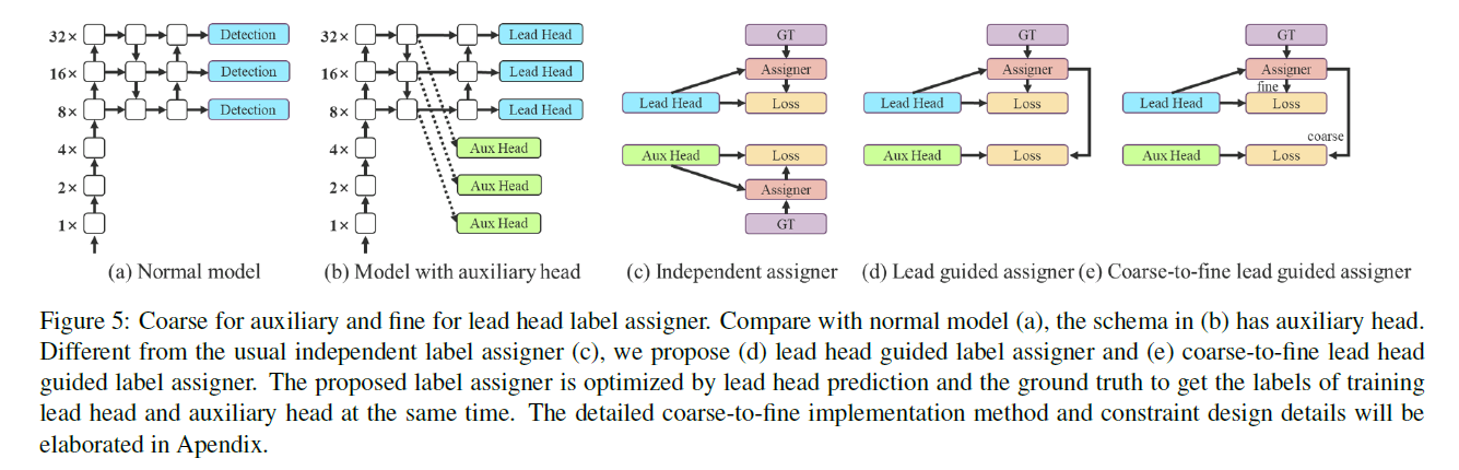
接下来我们要讨论label assignment的问题。在过去，在深度网络的训练过程中，label assignment通常是直接依据GT生成hard label，并按照预设规则进行分配。然而，近年来，以目标检测为例，研究者们往往会利用网络预测输出的质量和分布信息，再结合GT，通过一定的计算和优化方法来生成soft label。例如，YOLO使用预测框和真实框之间的IoU作为soft label。在这里，我们将这种同时考虑网络预测结果和GT，并据此分配soft label的机制称为label assigner。

那么我们该如何为lead head和auxiliary head分配soft label呢？据我们所知，目前尚未有相关文献探讨过这一问题。目前最常用的方法如Fig5(c)所示，即将lead head和auxiliary head分开，各自利用自身的预测结果和GT来进行label assignment。本文提出了一种新的label assignment方法，该方法利用lead head的预测结果来同时引导lead head和auxiliary head的训练，其包含两种不同的策略，见Fig5(d)和Fig5(e)。

👉Lead head guided label assigner

主要基于lead head的预测结果与GT进行计算，并通过优化过程生成soft label。这组soft label将同时用于训练lead head和auxiliary head。这样做的原因是lead head具有较强的学习能力，因此由其生成的soft label能够更好地反映源数据与目标之间的分布和相关性。此外，我们可以将这种学习方式视为一种广义的残差学习，通过让较浅层的auxiliary head直接学习lead head已经掌握的信息，lead head就能更专注于学习那些尚未被学习到的残差信息。

👉Coarse-to-fine lead head guided label assigner

同样基于lead head的预测结果与GT生成soft label。但是，在该过程中我们生成了两组不同的soft label，即coarse label和fine label。其中，fine label就是lead head的预测结果和GT直接生成的soft label，而coarse label则是在此基础上，放宽了对正样本标签的分配约束，即允许更多的grid被视为正样本。这样做的原因在于，auxiliary head的学习能力不如lead head强，为了避免遗漏需要学习的信息，我们在目标检测任务中更关注auxiliary head的recall优化，而对于lead head，我们则更关注precision的优化。

4.3.Other trainable bag-of-freebies

在训练中用到的一些BoF：

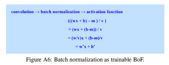
参考RepVGG，在推理阶段将BN层和卷积层进行融合。
YOLOR中的隐性知识。
仅在推理阶段使用EMA模型。注意，和Momentum梯度下降法不同，Momentum梯度下降法是对梯度更新使用EMA，而这里说的EMA模型是指更新模型参数的策略。详细来说，就是在YOLOv7训练一开始的时候，会复制一份当前模型作为EMA模型，之后每训练一个batch，就会按照EMA的策略对EMA模型的参数进行更新，注意，并不会影响原有模型的训练进程。这样得到的EMA模型更为稳定，鲁棒性更好。

5.Experiments

5.1.Experimental setup

使用COCO数据集进行实验。所有实验都没有使用预训练模型。也就是说，所有模型都是从头开始训练的。我们使用train 2017 set用于训练，val 2017 set用于验证和超参数选择。在test 2017 set上进行评估。详细的训练参数设置见Appendix。

我们设计了3种基础模型：

YOLOv7-tiny用于edge GPU。
YOLOv7用于normal GPU。
YOLOv7-W6用于cloud GPU。

通过对基础模型缩放，得到了许多变体，详见Appendix。需要注意的是，YOLOv7-tiny使用的是leaky ReLU作为激活函数。而其他模型使用SiLU作为激活函数。

5.2.Baselines

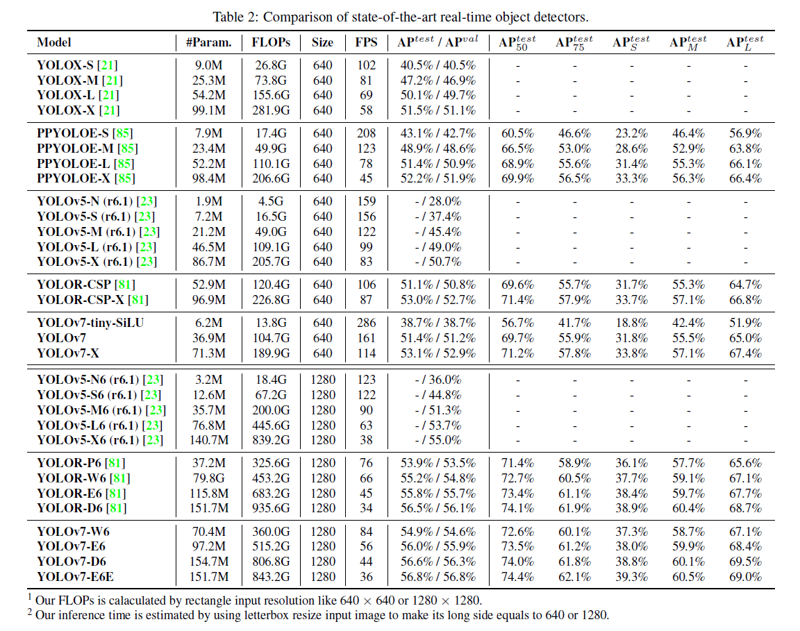
5.3.Comparison with state-of-the-arts

5.4.Ablation study

5.4.1.Proposed compound scaling method

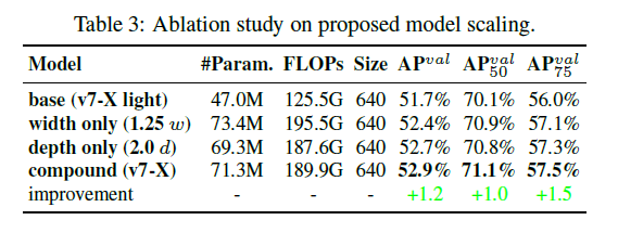
表3展示了模型缩放对性能的影响。第一行是base模型，第二行width only是仅将width扩大1.25倍，第三行depth only是仅将depth扩大2.0倍，第四行compound是将width扩大1.25倍的同时将depth扩大1.5倍。

5.4.2.Proposed planned re-parameterized model

为了验证我们所提出的重参数化方法的普适性。我们分别使用concatenation-based模型和residual-based模型用于验证。对于concatenation-based模型的验证，我们使用3个堆叠的ELAN；对于residual-based模型，我们使用CSPDarknet。

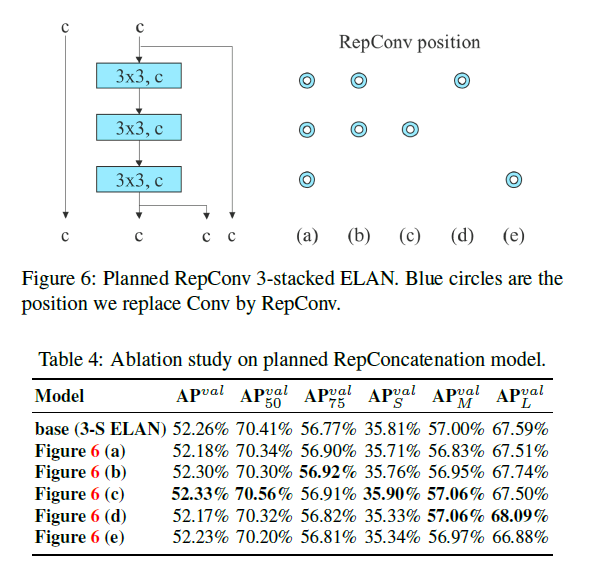
在验证concatenation-based模型时，我们将每个ELAN模块中的$3 \times 3$卷积层替换为RepConv。单个ELAN模块的结构如Fig6左图所示，和原始的ELAN结构有所不同，其中一条路径上有连续3个$3\times 3$卷积层，Fig6右图表示将对应位置的$3\times 3$卷积替换为RepConv。测试结果见表4。

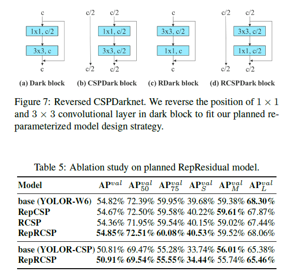
在验证residual-based模型时，如Fig7所示，Fig7(a)是原始的Darknet block，Fig7(b)是原始的CSPDarknet block。为了方便应用重参数化，将Darknet block和CSPDarknet block中的$3 \times 3$卷积挪到了$1 \times 1$卷积的前面，即Fig7(c)和Fig7(d)。测试结果见表5，其中RepCSP可参阅CSPRepResNet。

5.4.3.Proposed assistant loss for auxiliary head

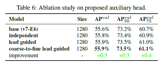
表6中的第二行“independent”表示的是lead head和auxiliary head各自采用独立的label assignment。

在Fig8中，Fig8(a)是输入图像，Fig8(b)和Fig8(c)指的是aux head和lead head的label assignment是各自独立的，Fig8(d)和Fig8(e)指的是第4.2部分提到的”Lead head guided label assigner”方式。以Fig8(b)为例，解释下如何看这个图。纵向”Pyramids”指的是金字塔feature map层级，横向”Anchors”指的是不同的3种anchor，所以说，$4 \times 3$中的每个格子都是一个objectness map，objectness map中每个grid的值越大（颜色越亮），就表示该grid存在object的可能性越大。

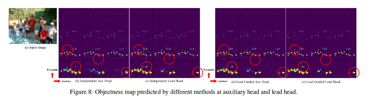
从Fig8的可视化结果可以看出，Lead Guided策略减少了噪声，提高了检测精度。

对于aux head，对于远离object中心的anchor box，我们可以将其objectness进行一个上限的限制。是否添加这个限制的测试结果见表7：

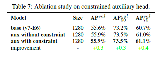
在表7中，”base”指的是基准模型，不加aux head。”aux without constraint”表示的是添加aux head，但没有objectness的限制。”aux with constraint”指的是添加aux head，并且有objectness的限制。

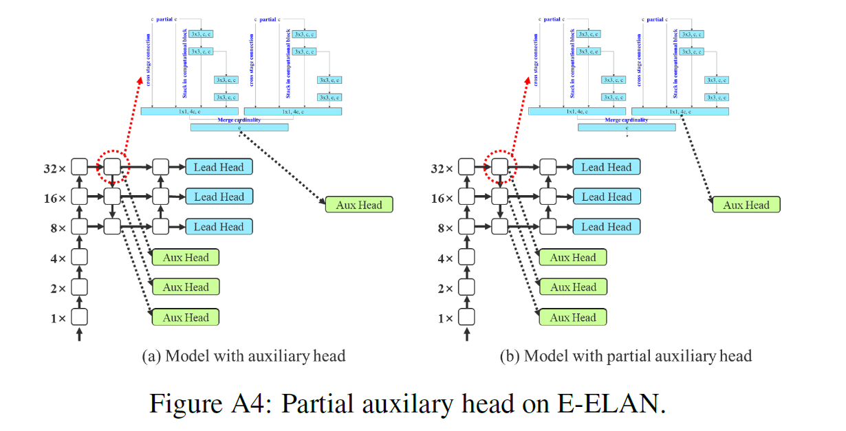
表8比较了”aux”和”partial aux”之间的性能区别：

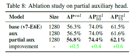
“aux”和”partial aux”的介绍见附录FigA4。

6.Conclusions

不再详述。

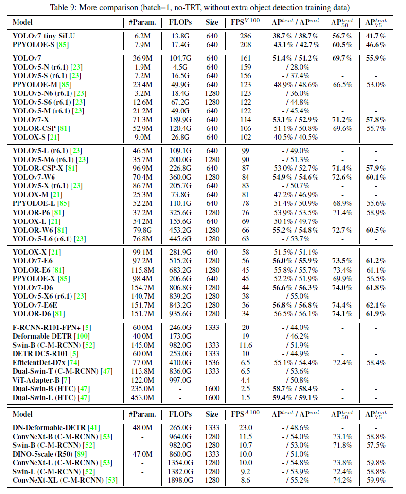
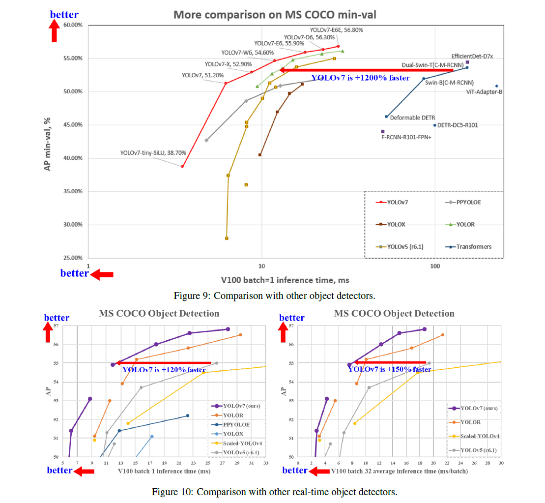
7.More comparison

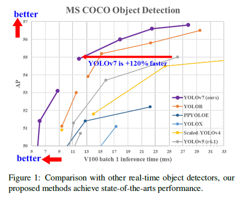
在5 FPS到160 FPS这个区间内，不管是精度还是速度，YOLOv7超过了所有已知的目标检测方法。

8.A.Appendix

8.A.1.Implementation details

8.A.1.1.Architectures

YOLOv7 P5的模型结构见FigA1：

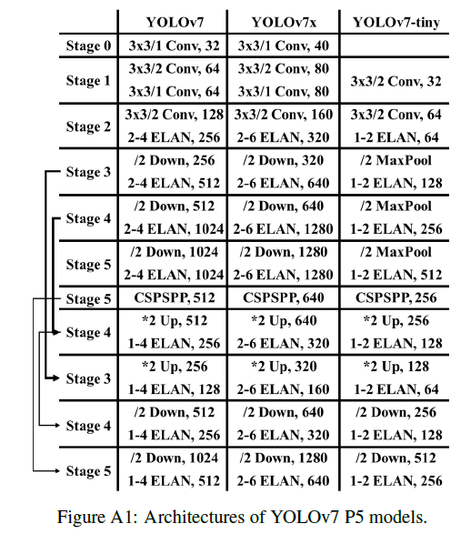
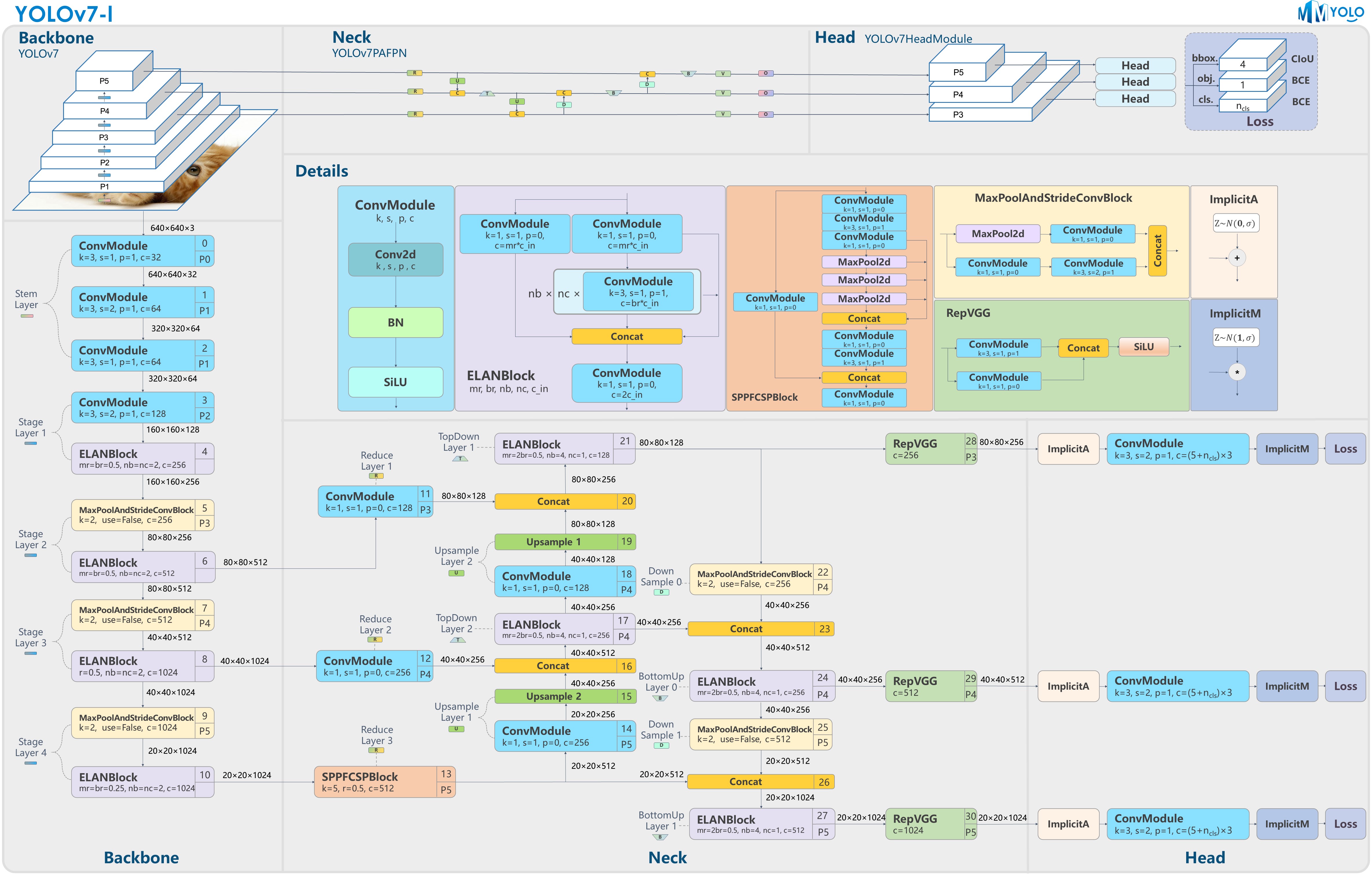
其中，YOLOv7的详细结构可参考下面两张图：

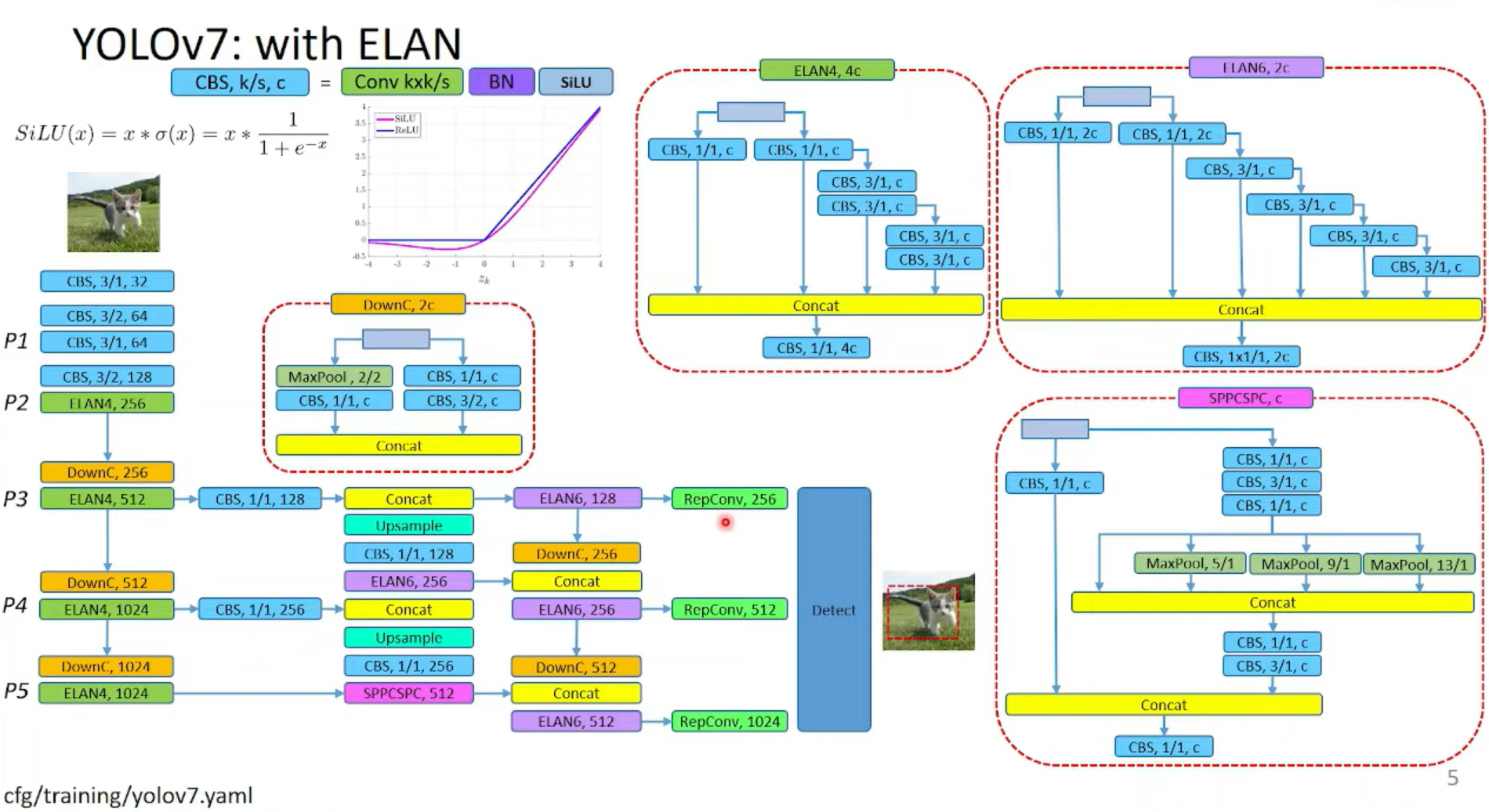
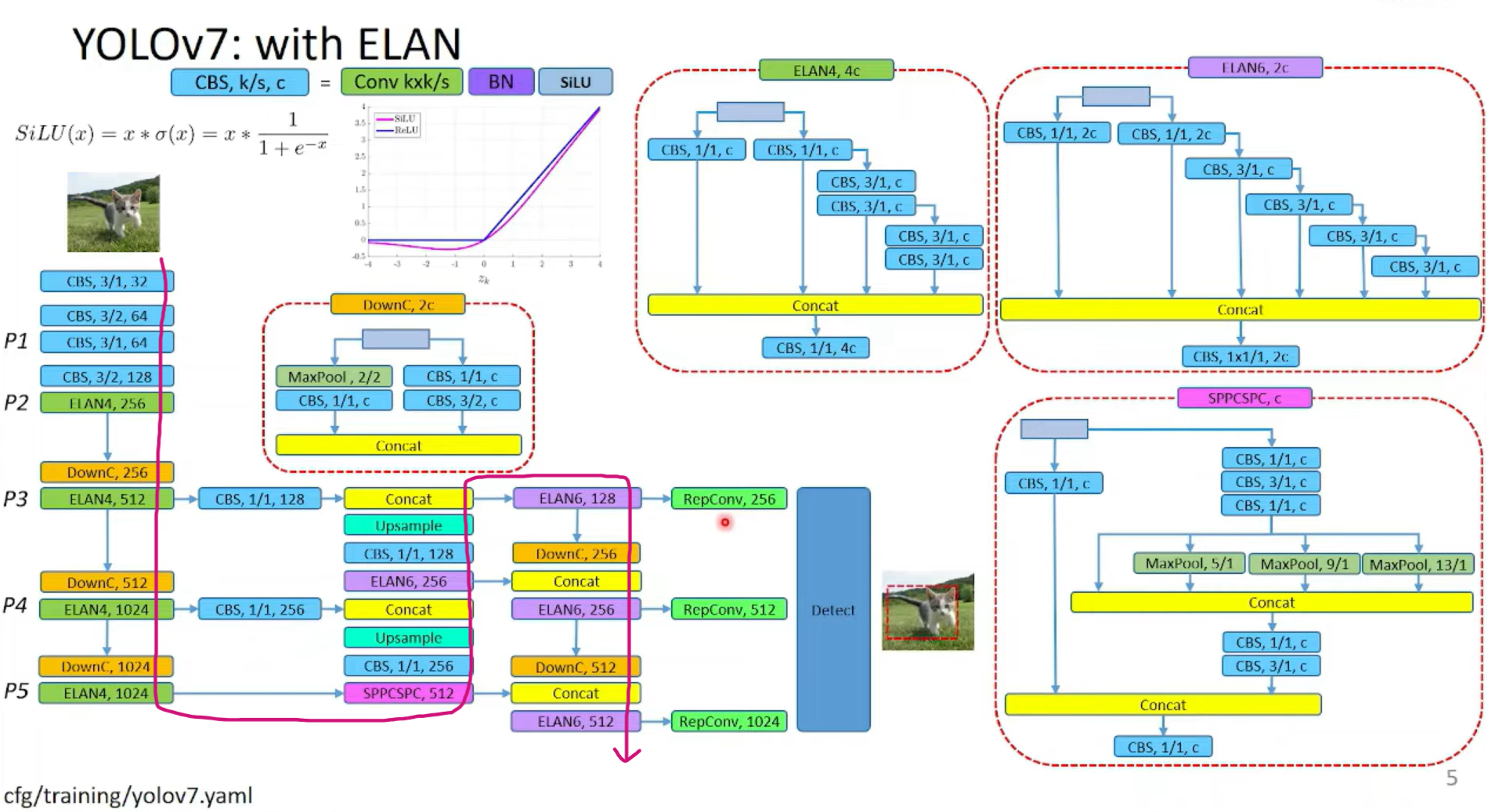
FigA1中的第一列YOLOv7是按照下图红色箭头所示的路径进行展示的：

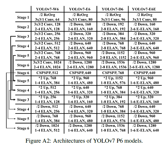
YOLOv7 P6的模型结构见FigA2：

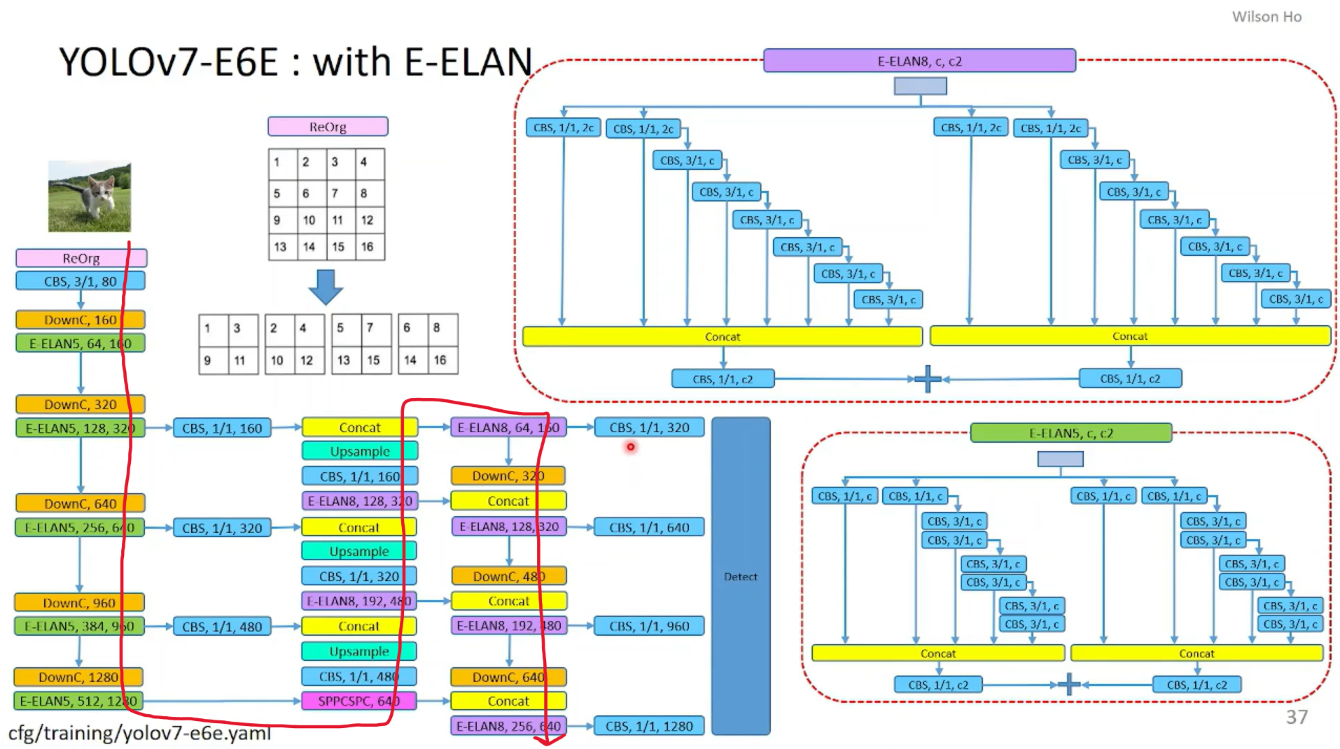
其中，YOLOv7-E6E的详细结构可参考下面这张图：

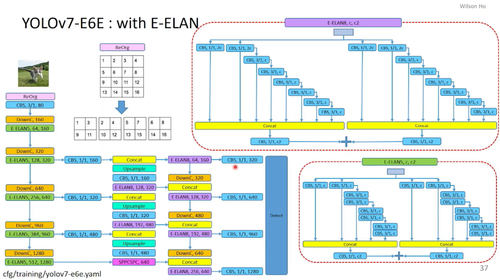
FigA2中的第四列YOLOv7-E6E是按照下图红色箭头所示的路径进行展示的：

在第3.1部分我们也提到过，对于E-ELAN框架，由于我们的edge devide不支持分组卷积和channel shuffle操作，所以采用了如FigA3(b)中的等价形式：

这种等价结构也使得我们更容易实现partial auxiliary head，如FigA4(b)所示。FigA4(a)是普通的auxiliary head。

接下来解释下第4.2部分提到的Coarse-to-fine lead head guided label assigner，即Fig5(e)所示的这种情况。

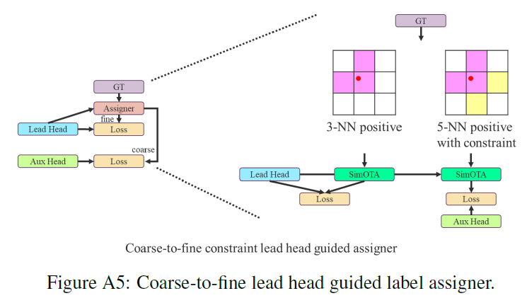
lead head和aux head都用到了SimOTA，FigA5中的3-NN positive和5-NN positive可参考在YOLOv4中对”Using multiple anchors for a single ground truth”部分的讲解，此处不再详述。对于lead head来说，3-NN positive就相当于是SimOTA中的fixed center area。对于aux head来说，其SimOTA的正样本搜索区域为fixed center area（即5-NN positive）、lead head的正样本以及GT box的并集。

8.A.1.2.Hyper-parameters

我们有3种不同的训练超参数设置。

👉第一种超参数设置：hyp.scratch.tiny.yaml，适用于YOLOv7-tiny。

lr0: 0.01  # initial learning rate (SGD=1E-2, Adam=1E-3)
lrf: 0.01  # final OneCycleLR learning rate (lr0 * lrf)
momentum: 0.937  # SGD momentum/Adam beta1
weight_decay: 0.0005  # optimizer weight decay 5e-4
warmup_epochs: 3.0  # warmup epochs (fractions ok)
warmup_momentum: 0.8  # warmup initial momentum
warmup_bias_lr: 0.1  # warmup initial bias lr
box: 0.05  # box loss gain
cls: 0.5  # cls loss gain
cls_pw: 1.0  # cls BCELoss positive_weight
obj: 1.0  # obj loss gain (scale with pixels)
obj_pw: 1.0  # obj BCELoss positive_weight
iou_t: 0.20  # IoU training threshold
anchor_t: 4.0  # anchor-multiple threshold
# anchors: 3  # anchors per output layer (0 to ignore)
fl_gamma: 0.0  # focal loss gamma (efficientDet default gamma=1.5)
hsv_h: 0.015  # image HSV-Hue augmentation (fraction)
hsv_s: 0.7  # image HSV-Saturation augmentation (fraction)
hsv_v: 0.4  # image HSV-Value augmentation (fraction)
degrees: 0.0  # image rotation (+/- deg)
translate: 0.1  # image translation (+/- fraction)
scale: 0.5  # image scale (+/- gain)
shear: 0.0  # image shear (+/- deg)
perspective: 0.0  # image perspective (+/- fraction), range 0-0.001
flipud: 0.0  # image flip up-down (probability)
fliplr: 0.5  # image flip left-right (probability)
mosaic: 1.0  # image mosaic (probability)
mixup: 0.05  # image mixup (probability)
copy_paste: 0.0  # image copy paste (probability)
paste_in: 0.05  # image copy paste (probability), use 0 for faster training
loss_ota: 1 # use ComputeLossOTA, use 0 for faster training

👉第二种超参数设置：hyp.scratch.p5.yaml，适用于YOLOv7和YOLOv7x。

lr0: 0.01  # initial learning rate (SGD=1E-2, Adam=1E-3)
lrf: 0.1  # final OneCycleLR learning rate (lr0 * lrf)
momentum: 0.937  # SGD momentum/Adam beta1
weight_decay: 0.0005  # optimizer weight decay 5e-4
warmup_epochs: 3.0  # warmup epochs (fractions ok)
warmup_momentum: 0.8  # warmup initial momentum
warmup_bias_lr: 0.1  # warmup initial bias lr
box: 0.05  # box loss gain
cls: 0.3  # cls loss gain
cls_pw: 1.0  # cls BCELoss positive_weight
obj: 0.7  # obj loss gain (scale with pixels)
obj_pw: 1.0  # obj BCELoss positive_weight
iou_t: 0.20  # IoU training threshold
anchor_t: 4.0  # anchor-multiple threshold
# anchors: 3  # anchors per output layer (0 to ignore)
fl_gamma: 0.0  # focal loss gamma (efficientDet default gamma=1.5)
hsv_h: 0.015  # image HSV-Hue augmentation (fraction)
hsv_s: 0.7  # image HSV-Saturation augmentation (fraction)
hsv_v: 0.4  # image HSV-Value augmentation (fraction)
degrees: 0.0  # image rotation (+/- deg)
translate: 0.2  # image translation (+/- fraction)
scale: 0.9  # image scale (+/- gain)
shear: 0.0  # image shear (+/- deg)
perspective: 0.0  # image perspective (+/- fraction), range 0-0.001
flipud: 0.0  # image flip up-down (probability)
fliplr: 0.5  # image flip left-right (probability)
mosaic: 1.0  # image mosaic (probability)
mixup: 0.15  # image mixup (probability)
copy_paste: 0.0  # image copy paste (probability)
paste_in: 0.15  # image copy paste (probability), use 0 for faster training
loss_ota: 1 # use ComputeLossOTA, use 0 for faster training

👉第三种超参数设置：hyp.scratch.p6.yaml，适用于YOLOv7-W6、YOLOv7-E6、YOLOv7-D6和YOLOv7-E6E。

lr0: 0.01  # initial learning rate (SGD=1E-2, Adam=1E-3)
lrf: 0.2  # final OneCycleLR learning rate (lr0 * lrf)
momentum: 0.937  # SGD momentum/Adam beta1
weight_decay: 0.0005  # optimizer weight decay 5e-4
warmup_epochs: 3.0  # warmup epochs (fractions ok)
warmup_momentum: 0.8  # warmup initial momentum
warmup_bias_lr: 0.1  # warmup initial bias lr
box: 0.05  # box loss gain
cls: 0.3  # cls loss gain
cls_pw: 1.0  # cls BCELoss positive_weight
obj: 0.7  # obj loss gain (scale with pixels)
obj_pw: 1.0  # obj BCELoss positive_weight
iou_t: 0.20  # IoU training threshold
anchor_t: 4.0  # anchor-multiple threshold
# anchors: 3  # anchors per output layer (0 to ignore)
fl_gamma: 0.0  # focal loss gamma (efficientDet default gamma=1.5)
hsv_h: 0.015  # image HSV-Hue augmentation (fraction)
hsv_s: 0.7  # image HSV-Saturation augmentation (fraction)
hsv_v: 0.4  # image HSV-Value augmentation (fraction)
degrees: 0.0  # image rotation (+/- deg)
translate: 0.2  # image translation (+/- fraction)
scale: 0.9  # image scale (+/- gain)
shear: 0.0  # image shear (+/- deg)
perspective: 0.0  # image perspective (+/- fraction), range 0-0.001
flipud: 0.0  # image flip up-down (probability)
fliplr: 0.5  # image flip left-right (probability)
mosaic: 1.0  # image mosaic (probability)
mixup: 0.15  # image mixup (probability)
copy_paste: 0.0  # image copy paste (probability)
paste_in: 0.15  # image copy paste (probability), use 0 for faster training
loss_ota: 1 # use ComputeLossOTA, use 0 for faster training

此外，还有一个额外的超参数top k用于SimOTA。在训练$640\times 640$模型时，设置$k=10$。在训练$1280 \times 1280$模型时，设置$k=20$。

8.A.1.3.Re-parameterization

可参考RepVGG，将“卷积-BN-激活函数”重参数化为“卷积-激活函数”的公式见FigA6：

FigA7展示了在YOLOR中，如何将隐性知识合并在卷积中（个人理解：应该也是应用在推理阶段）：

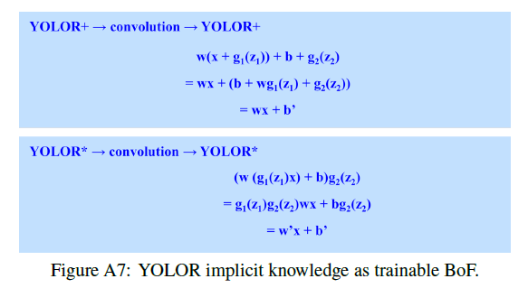
在FigA7上图中，先是加操作的隐性知识，然后执行卷积，接着又是一个加操作的隐性知识。在FigA7下图中，先是乘操作的隐性知识，然后执行卷积，接着又是一个乘操作的隐性知识。

8.A.2.More results

8.A.2.1.YOLOv7-mask

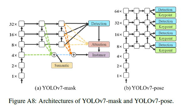
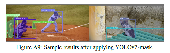
我们集成了YOLOv7和BlendMask用于实例分割。我们只是简单的将YOLOv7目标检测模型在MS COCO实例分割数据集上训练了30个epoch。它就达到了SOTA的实时实例分割结果。YOLOv7-mask的模型框架见FigA8(a)，一些检测结果见FigA9。

BlendMask论文：Chen et al. BlendMask: Top-down meets bottom-up for instance segmentation. CVPR, 2020.。

8.A.2.2.YOLOv7-pose

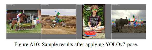
我们集成了YOLOv7和YOLO-Pose用于关键点检测。我们遵循和YOLO-Pose一样的设置，将YOLOv7-W6人体关键点检测模型在MS COCO关键点检测数据集上进行fine-tune。YOLOv7-W6-pose达到了SOTA的实时人体姿态估计结果。YOLOv7-W6-pose的模型框架见FigA8(b)，一些检测结果见FigA10。

YOLO-Pose论文：Maji et al. YOLO-Pose: Enhancing YOLO for Multi Person Pose Estimation Using Object Keypoint Similarity Loss. CVPRW, 2022.。

9.原文链接

👽YOLOv7：Trainable bag-of-freebies sets new state-of-the-art for real-time object detectors

【论文阅读】YOLOv7：Trainable bag-of-freebies sets new state-of-the-art for real-time object detectors

YOLOv7